Gallery of plots and scripts 1. Synchrotron sources

Synchrotron sources

The images below are produced by \tests\raycing\test_sources.py and by \examples\withRaycing\01_SynchrotronSources\synchrotronSources.py.

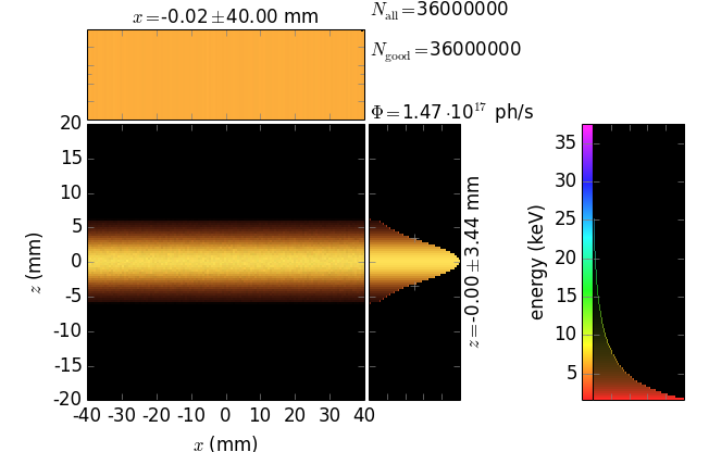
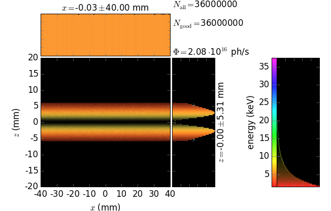
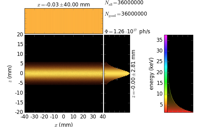
Bending magnet

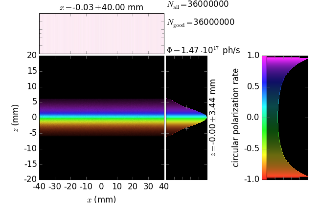
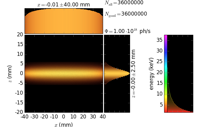
On a transversal screen the image is unlimited horizontally (practically limited by the front end). The energy distribution is red-shifted for off-plane photons. The polarization is primarily horizontal. The off-plane radiation has non-zero projection to the vertical polarization plane.

source	total flux	horiz. pol. flux	vert. pol. flux
using WS
internal xrt

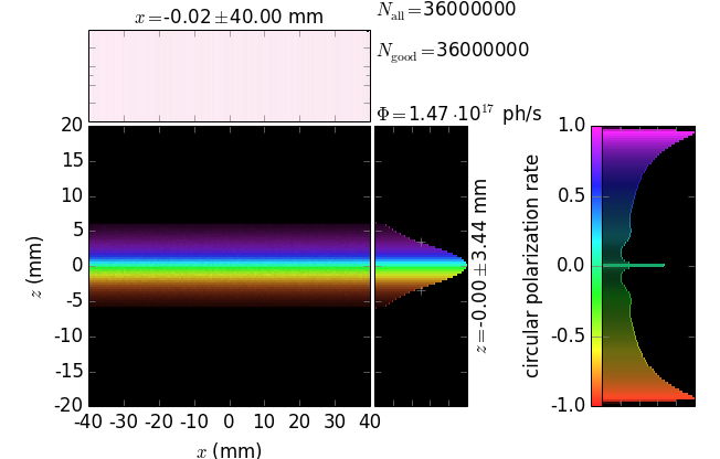
The off-plane radiation is in fact left and right polarized:

source	circular polarization rate
using WS
internal xrt

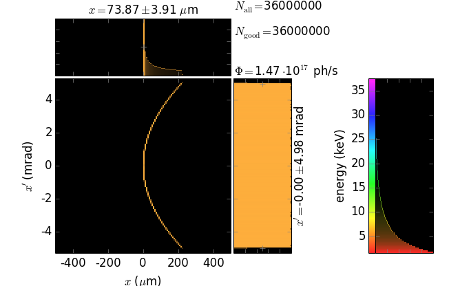
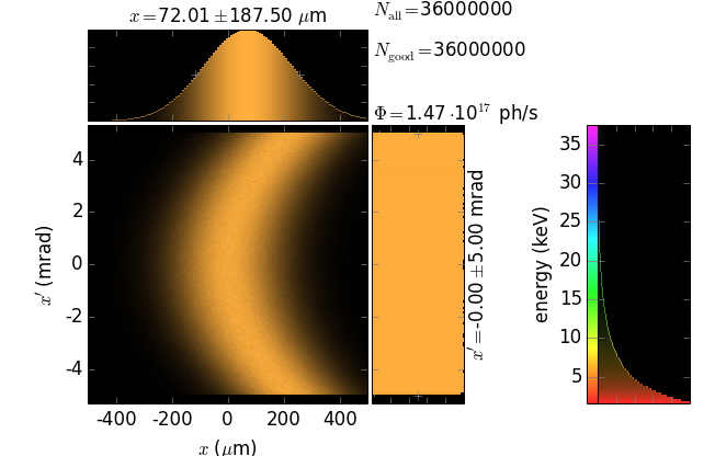
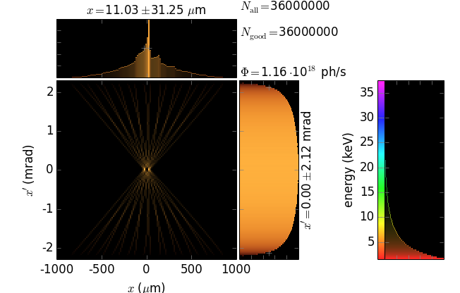
The horizontal phase space projected to a transversal plane at the origin is parabolic:

zero electron beam size	σx = 49 µm

Multipole wiggler

The horizontal image size is determined by the parameter K. The energy distribution is red-shifted for off-plane photons. The polarization is primarily horizontal. The off-plane radiation has non-zero projection to the vertical polarization plane.

source	total flux	horiz. pol. flux	vert. pol. flux
using WS
internal xrt

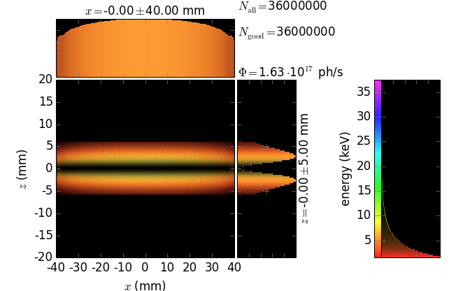
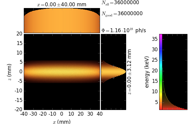
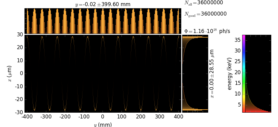
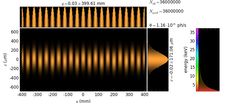
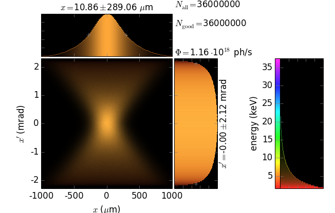
The horizontal longitudinal cross-section reveals a sinusoidal shape of the source. The horizontal phase space projected to the transversal plane at the origin has individual branches for each pole.

zero electron beam size	σx = 49 µm

Undulator

The module test_sources has functions for visualization of the angular and energy distributions of the implemented sources in 2D and 3D. This is especially useful for undulators because they have sharp peaks, which requires a proper selection of angular and energy meshes.

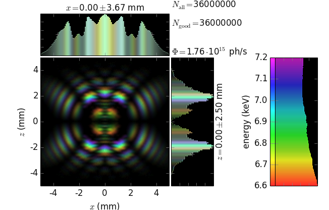
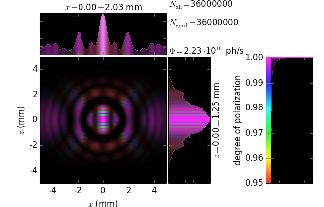
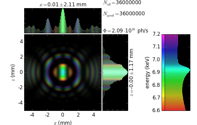
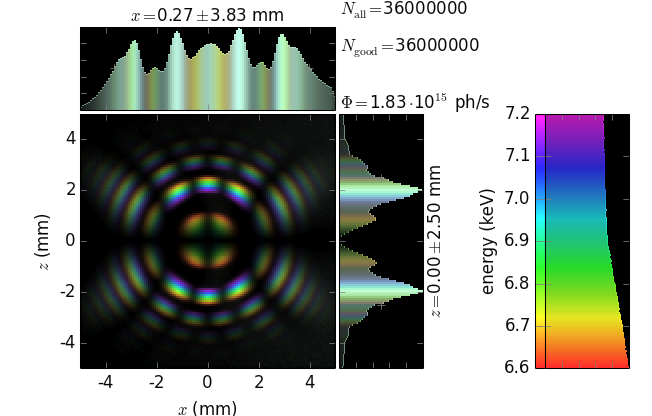
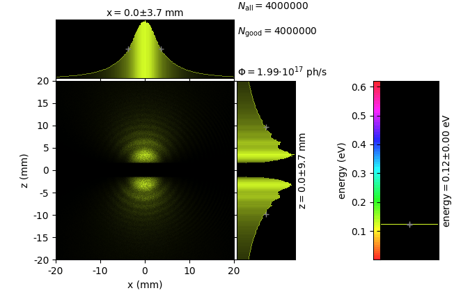
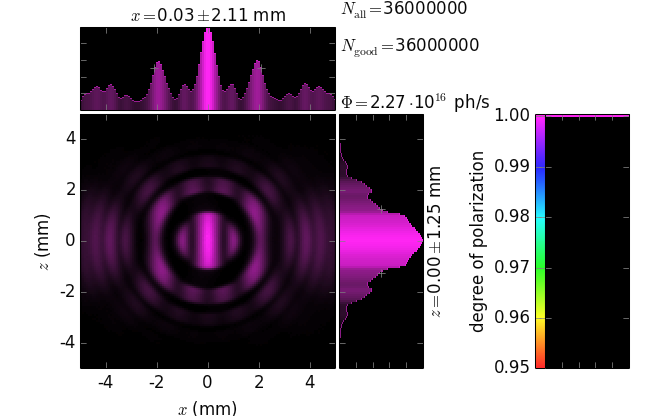
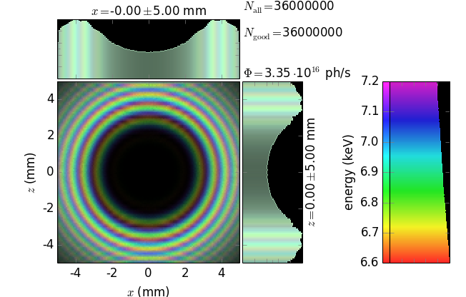
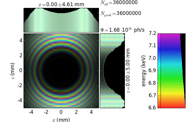
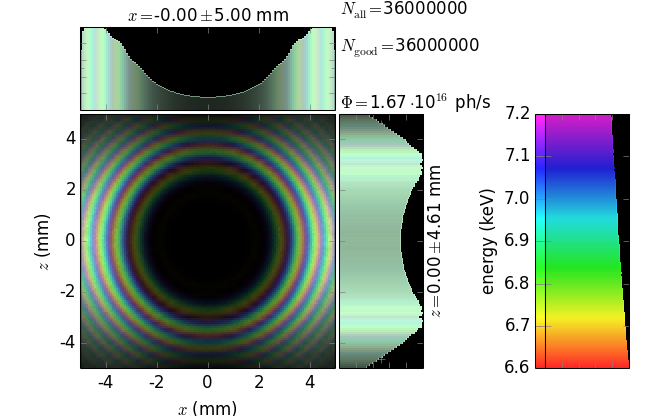
The ray traced images of an undulator source (produced by \examples\withRaycing\01_SynchrotronSources\synchrotronSources.py) are feature-rich. The polarization is primarily horizontal. The off-plane radiation has non-zero projection to the vertical polarization plane.

source	total flux	hor. pol. flux	ver. pol. flux	deg. of pol.
using Urgent
xrt

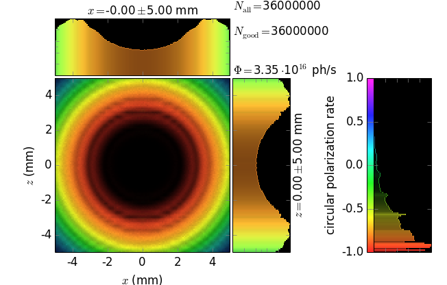
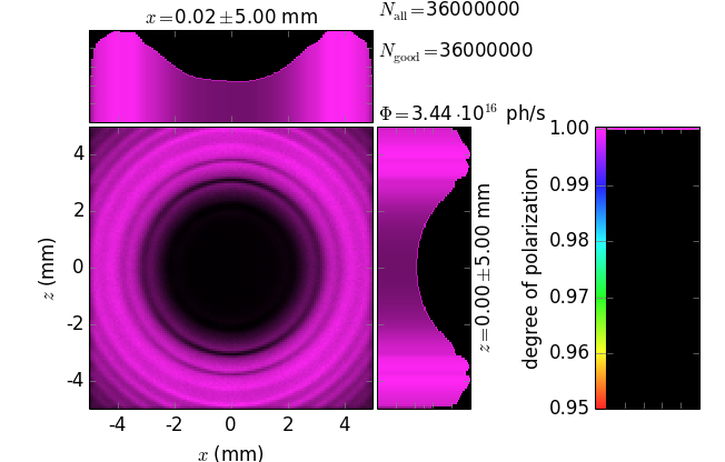
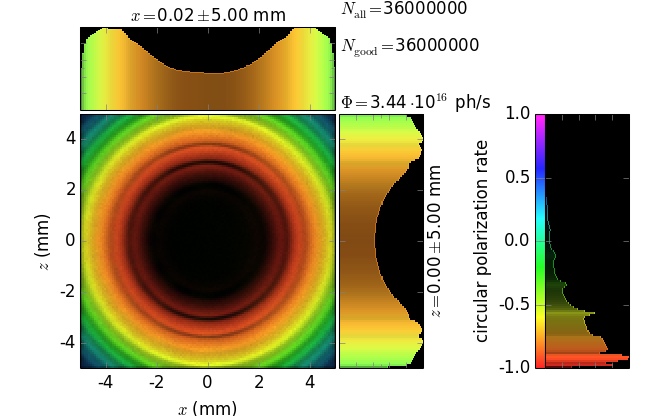
Elliptical undulator

An elliptical undulator gives circular images with a higher circular polarization rate in the inner rings:

source	total flux	hor. pol. flux	ver. pol. flux
using Urgent
internal xrt

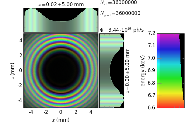
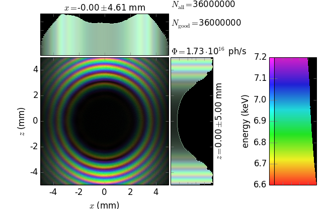
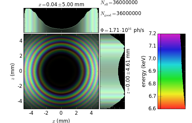
source	deg. of pol.	circular polarization rate
using Urgent
internal xrt

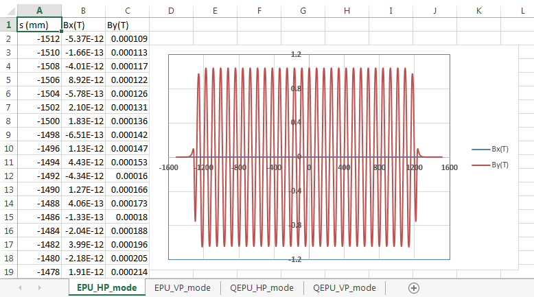
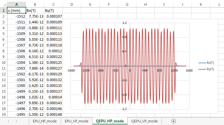
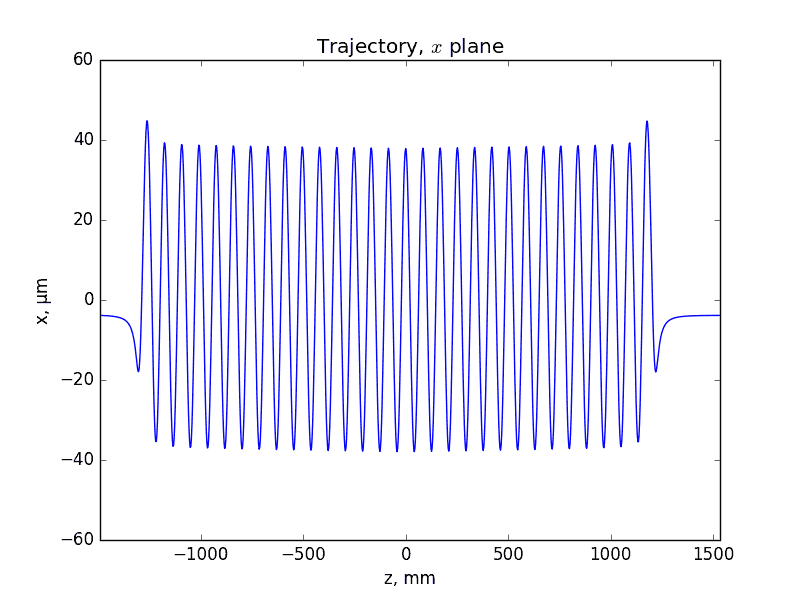
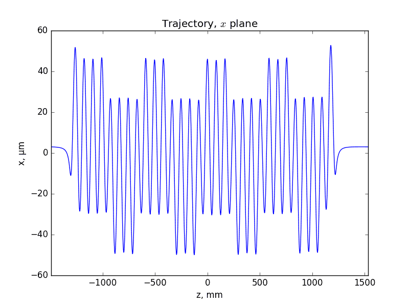
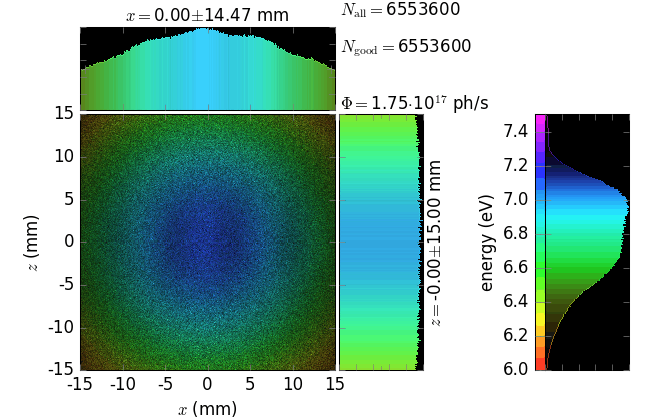
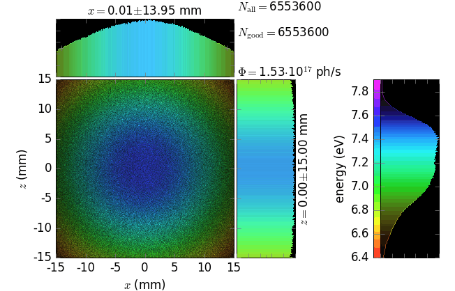
Custom field undulator

A custom magnetic field can be specified by an Excel file or a column text file. The example below is based on a table supplied by Hamed Tarawneh [Tarawneh]. The idea of introducing quasi-periodicity is to shift the n-th harmonics down in energy relative to the exact n-fold multiple of the 1st harmonic energy. This trick eliminates higher monochromator harmonics that are situated at the exact n-fold energies, which is a safer solution compared to a gas absorption filter.

Compare the harmonic energies (half-maximum position at the higher energy side) of the 3rd harmonic with the triple energy of the 1st harmonic.

[Tarawneh]

Quasi-periodic undulator field for ARPES beamline at MAX IV 1.5 GeV ring, (2016) unpublished.

Note

The definition of xyz coordinate system differs for the tabulated field and for xrt screens: z is along the beam direction in the tabulation and as a vertical axis in xrt.

	periodic	quasi-periodic
tabulated field
trajectory top view
wide band image and spectrum
1st harmonic image and spectrum
3rd harmonic image and spectrum

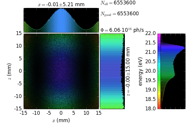
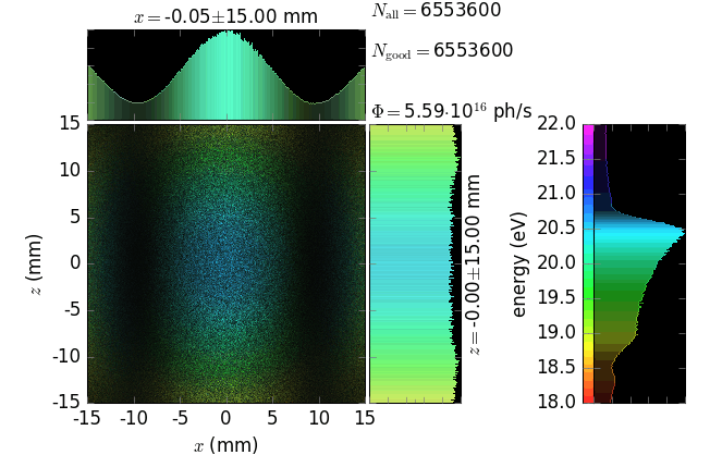
For validation, our calculations are compared here with those by Spectra for a particular case — quasi-periodic undulator defined by the same tabulated field, the 3rd harmonic, at E=20.5 eV. Notice again that Spectra provides either a spectrum or a transverse image while xrt can combine both by using colors and brightness. Notice also that on the following pictures the p-polarized flux is only ~3% of the total flux.

	SPECTRA	xrt
total flux
p-pol flux

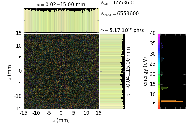
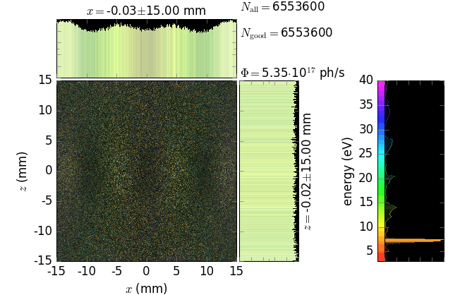
Infrared edge radiation

The images below are produced by examples/withRaycing/01_SynchrotronSources/edge_radiation.py.

This example calculates an infrared source consisting of two bending magnets defined by a big table of magnetic field. The magnetic field has four narrow ranges of rapid field change, so called field edges, where edge radiation is born. The two inner regions are aligned along the straight section, and their radiation enters the beamline front end. The outer two edges produce radiation that is directed to extreme negative and positive angles relative to the straight section.

magnetic field	electron beam trajectory

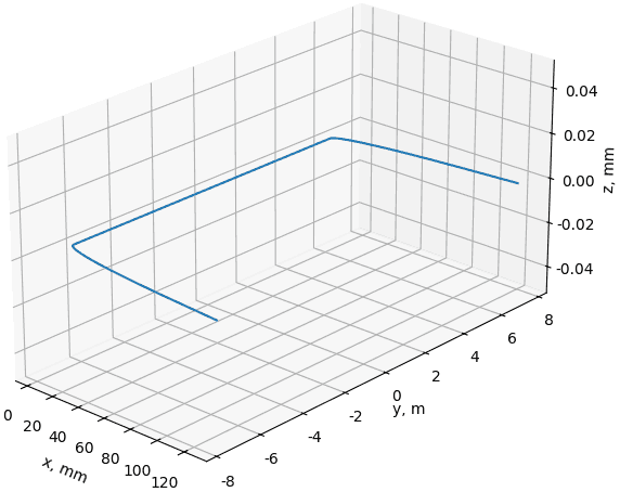
The infrared wavelength in this example is 10 µm. The equatorial gap mimics a 3 mm gap in the extracting mirror that reflects the beam sideways or upwards. The calculated field also containes bending magnet radiation that is about two orders of magnitude weaker than edge radiation at this energy and therefore is not visible on the pictures below.

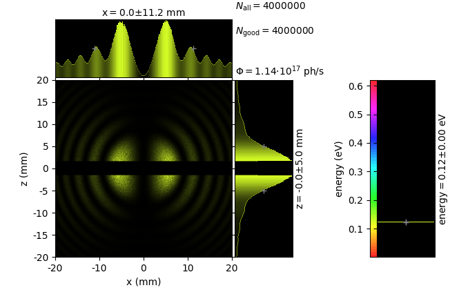
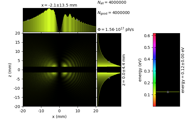
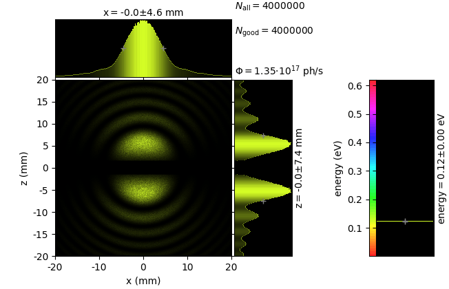
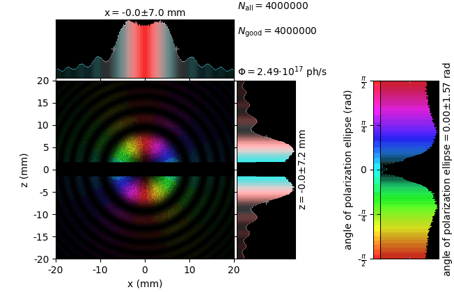
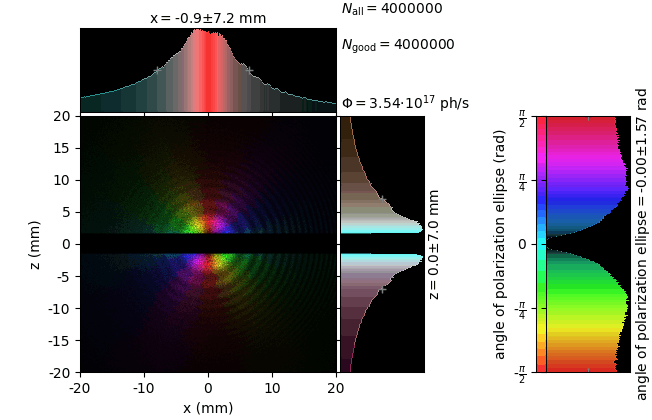
Edge radiation has a peculiar polarization pattern: it is radially polarized [Bosch]. This property is demonstrated by the polarization selective images in the table below: the p-polarized image is suppressed in the equatorial region whereas the s-polarized image is suppressed in the vertical meridional region. The lowest images, colored by the polarization ellipse angle, additionally demonstrate the radial polarization property.

This example is an extreme case of a difference between far field and near field calculation expressions, compare the two columns.

[Bosch]

Focusing of infrared edge and synchrotron radiation, NIMA 431 (1999) 320–333

	far field	near field
s-pol
p-pol
pol ellipse angle

Undulator radiation through rectangular aperture

The images below are produced by \examples\withRaycing\01_SynchrotronSources\fluxThroughAperture.py.

This example illustrates the sampling concepts explained in Section Sampling strategies.

Grid sampling comes in two flavors: with a grid exactly matching the 100×100 µrad² aperture and with the same grid plus extra 30% margins on each side. Adding margins is crucial for doing convolution with electron beam angular spread. Notice that for the sharp field distributions at zero emittance and zero energy spread, the grid has to be set with fine angular steps, otherwise the flux density spectrum gets unreal ripples. One may play with ntheta and npsi values to observe the effect.

In this particular example (MAX IV Linac), eEspread value is four times bigger than a typical value for a storage ring and so the grid here needs a bigger number of gamma (relative electron beam energy) samples to obtain a smooth spectrum. One may play with eSpreadNSamples parameter to observe the effect.

Ray tracing examples illustrate two different ways of field sampling: uniform reciprocal space sampling and sampling by intensity distribution. Energy can also be sampled variously: uniformly within a given range and on an equidistant mesh (energy scan). The latter case also delivers single energy field images, which also has some calculation overhead.

The following cases are sorted in increased complexity (and calculation time) from top to bottom.

Zero emittance, zero energy spread. Here, angular mesh has to be very dense due to very sharp field features.
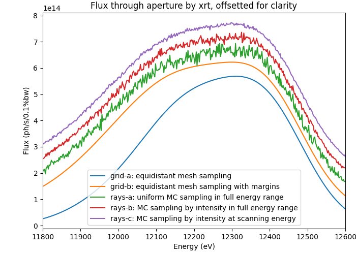
Non-zero emittance, zero energy spread. Here, extra margins have to be added to the angular mesh in order to be able to convolve with electron beam divergence. In this example, adding 30% margins (the orange curve) was not enough.
Non-zero emittance, non-zero energy spread. Here, the number of energy spread samples has to be adjusted for a large energy spread sigma otherwise the spectrum may have false sharp peaks.

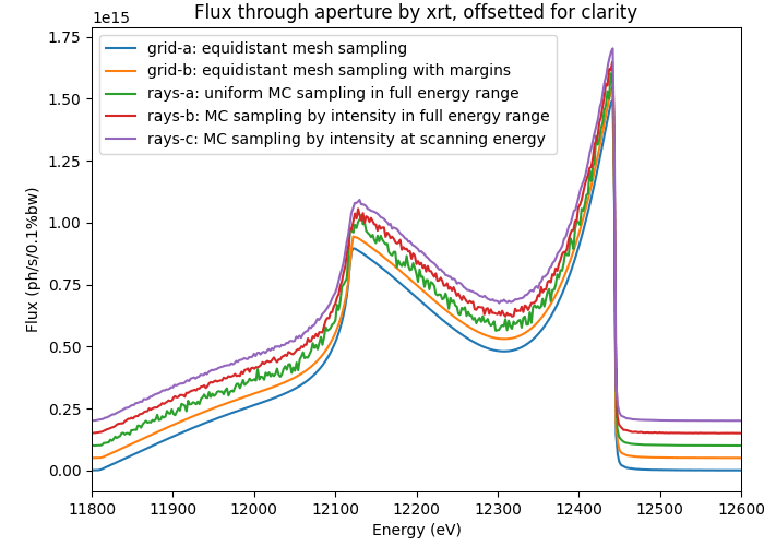
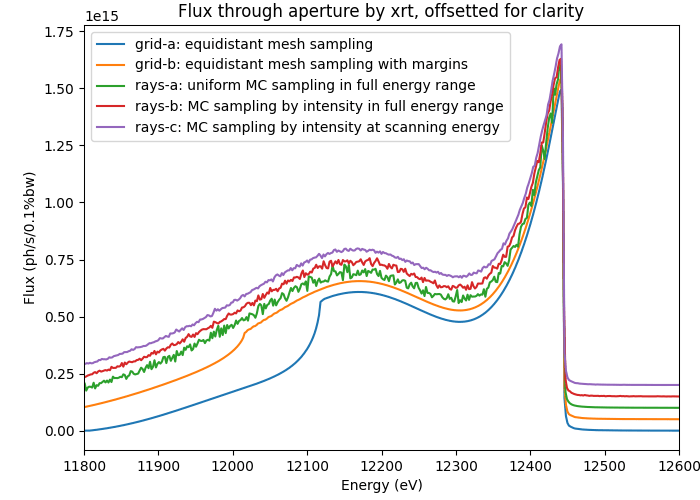
Finally, the standard ray tracing approach (“rays-b”) should be the method of choice as it does not need any parameter adjustment (in contrast to the grid methods). For not extreme cases (not too small aperture or not to big emittance and not too big energy spread) grid methods can be most efficient but anyways need a sanity check by ray tracing.

Orbital Angular Momentum of helical undulator radiation

The images below are produced by \examples\withRaycing\01_SynchrotronSources\undulatorVortex.py.

This example calculates flux and Orbital Angular Momentum (OAM) of helical undulator radiation. The calculation is done on a 3D (energy, theta, psi) or 4D (energy, theta, psi, gamma) rectangular mesh for zero and true electron beam energy spread, respectively. To calculate OAM projection along the propagation direction, we first calculate OAM intensity \(I^l_s\) for the field \(E_s\)

\[I^l_s = E_s^* i\left(\psi\frac{\partial}{\partial\theta}- \theta\frac{\partial}{\partial\psi}\right) E_s\]

and similarly for the field \(E_p\). OAM intensity is an incoherent distribution, similarly to the “usual” intensity, as the phase information is lost in it, and therefore it is suitable for incoherent accumulation of fields originated from different electrons distributed within emittance and energy spread distributions. After averaging intensity and OAM intensity over electron beam energy spread distribution and convolving with electron beam angular distributions, we obtain vorticity – the averaged normalized OAM value:

\[l_s = \int I^l_s d\theta d\psi \bigg/ \int I_s d\theta d\psi\]

and similarly for the field \(E_p\).

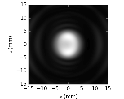
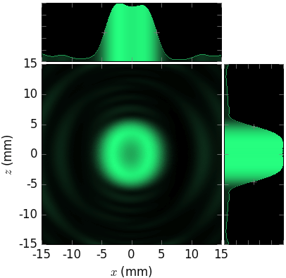
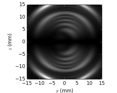
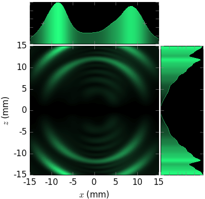
The images below were calculated at the maximum flux energies at the 1st to 4th harmonics. As a reminder, the flux is maximized at energies slightly below the formal harmonic energies; at these energies the transverse distribution is of a donut shape. As a second reminder, the radiation from a helical undulator has only the first harmonic on the undulator axis but also has higher harmonics at finite observation angles.

The coloring of the transverse images is done by field phase. For this purpose, the radiation field (here, \(E_s\)) was coherently averaged over electron beam energy spread distribution and electron beam angular distributions. This operation is physically illegal but was used here only for the visual effect. The measurable values – intensity, flux and vorticity – were determined by the correct incoherent averaging. The image brightness represents intensity.

	zero emittance, zero energy spread	true emittance, true energy spread
Flux and vorticity
1st harmonic
2nd harmonic
3rd harmonic
4th harmonic

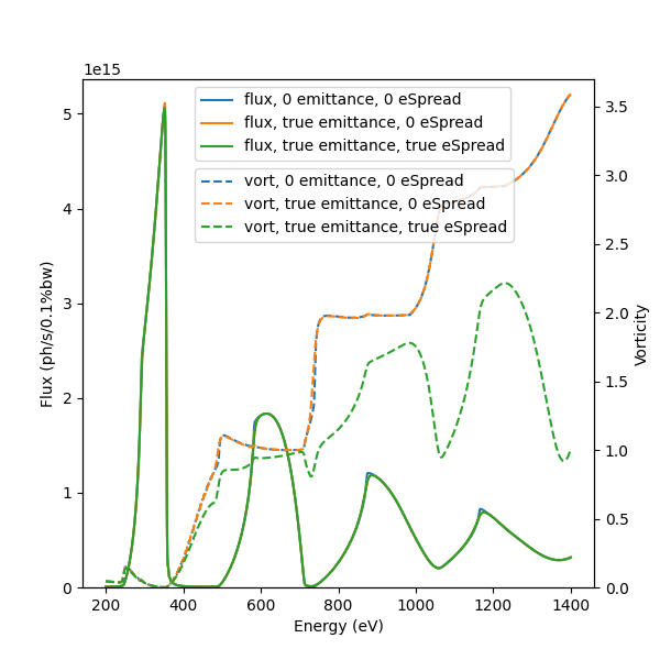
As expected, vorticity approximately equals the harmonic number minus one in the perfect case of zero emittance and zero energy spread. This pattern is quite strongly affected by electron beam energy spread. Emittance plays a much lesser role as the used angular acceptance is much bigger than the electron beam angular distributions (360 µrad vs 5.8 and 2.0 µrad rms).