Gallery of plots and scripts 3. Wave propagation

These examples are based on wave diffraction via Kirchhoff integral.

Warning

You need a good graphics card for running these calculations!

Note

Consider the warnings and tips on using xrt with GPUs.

Diffraction from mirror surface

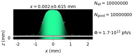
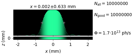
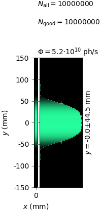
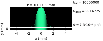
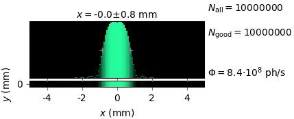
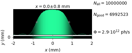
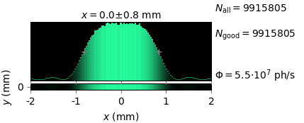
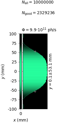
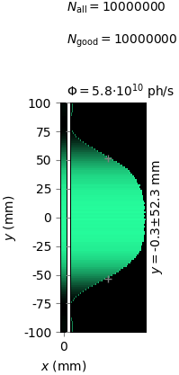
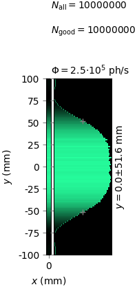
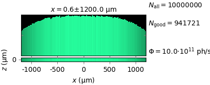
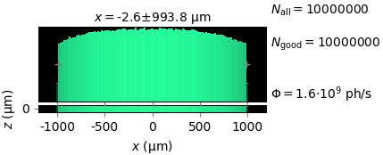
This example shows wave diffraction from a geometric source onto a flat or hemispheric screen. The source is rectangular with no divergence. The mirror has no material properties (reflectivity is 1) for simplicity. Notice the difference in the calculated flux between the rays and the waves.

rays	wave

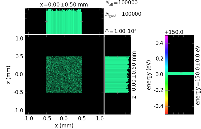
The flux losses are not due to the integration errors, as was proven by variously dense meshes. The losses are solely caused by cutting the tails, as proven by a wider image shown below.

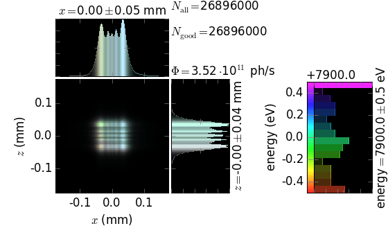
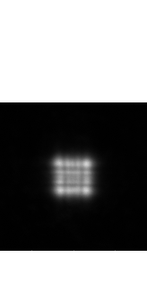
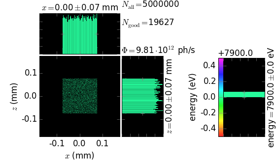
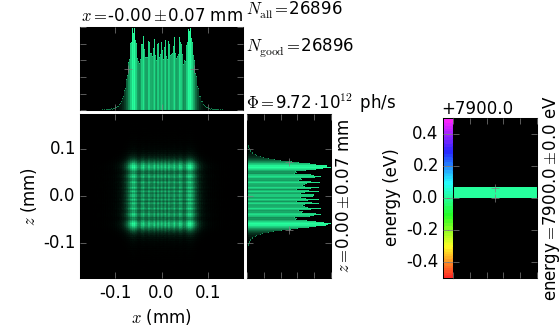
Slit diffraction with undulator source

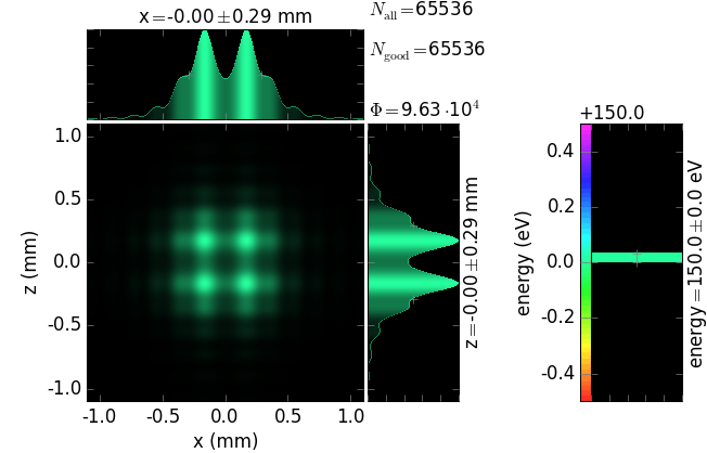
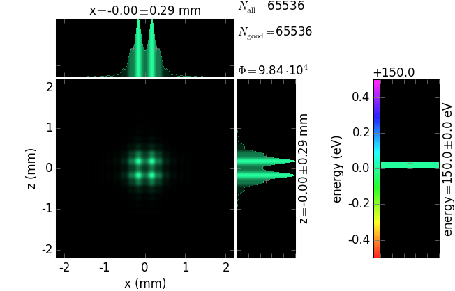
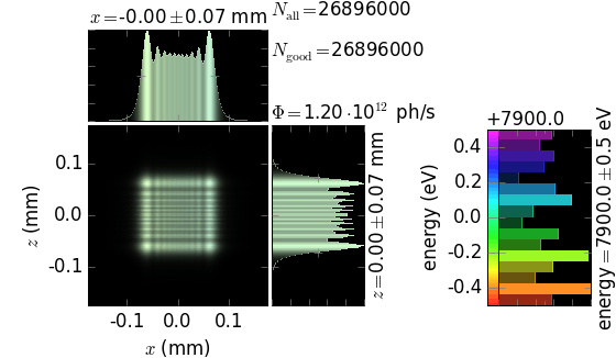
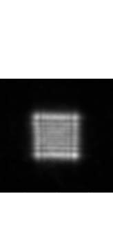
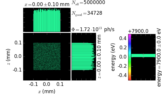
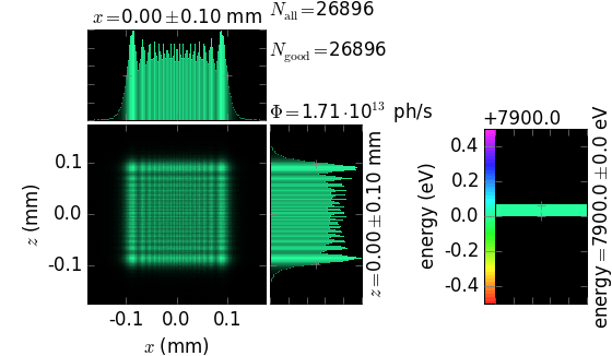
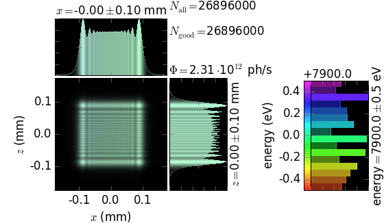
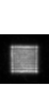
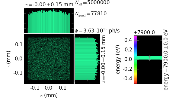
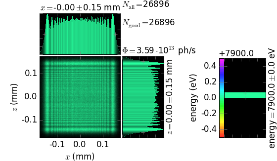
This example shows wave diffraction of an undulator beam on a square slit. The calculations were done for (1) a monochromatic beam with zero electron beam emittance and (2) a finite energy band beam with the real electron emittance of Petra III ring. The resulted images are compared with experimentally measured ones [Zozulya_Sprung].

Notice that vertical stripes are less pronounced in the complete calculations because the horizontal emittance is much larger than the vertical one.

[Zozulya_Sprung]

A. Zozulya and M. Sprung, measured at P10 beamline, DESY Photon Science (2014) unpublished.

slit size (µm²)	ray tracing, zero emittance	diffraction, zero emittance	diffraction, real emittance	exp P10
100×100
150×150
200×200
300×300

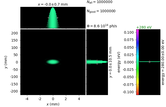
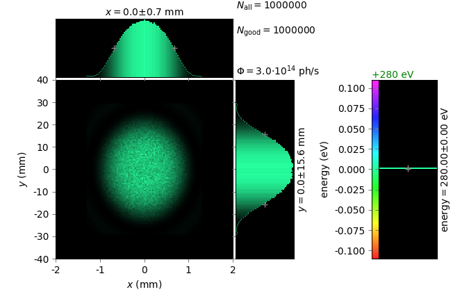
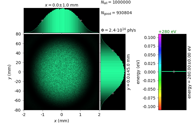
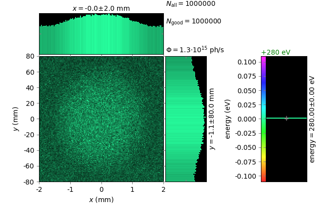
Young’s experiment with undulator source

This example shows double slit diffraction of an undulator beam. The single slit width is 10 µm, the slit separation is variable (displayed is edge-to-edge distance), the slit position is 90 m from the source and the screen is at 110 m.

Diffraction from grating

Various gratings described in [Boots] have been tested with xrt for diffraction efficiency. The efficiency curves in [Boots] were calculated by means of the code peg which provides almost identical results to those by REFLEC [REFLEC] but with reportedly better convergence. In order to have comparison curves, we got the REFLEC results calculated by R. Sankari [Sankari] which were basically equal to those in [Boots].

[Boots]

(1, 2, 3, 4) M. Boots, D. Muir and A. Moewes, Optimizing and characterizing grating efficiency for a soft X-ray emission spectrometer, J. Synchrotron Rad. 20 (2013) 272–285.

[REFLEC]

F. Schäfers and M. Krumrey, Technischer Bericht, BESSY TB 201 (1996).

[Sankari]

Sankari, private communication (2015).

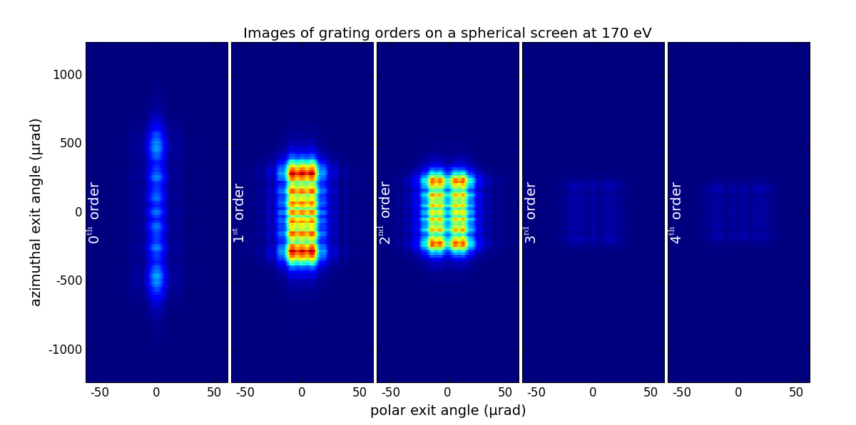
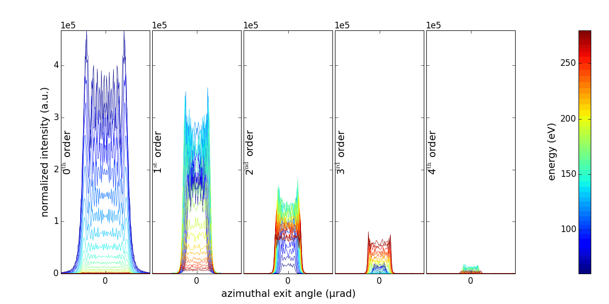
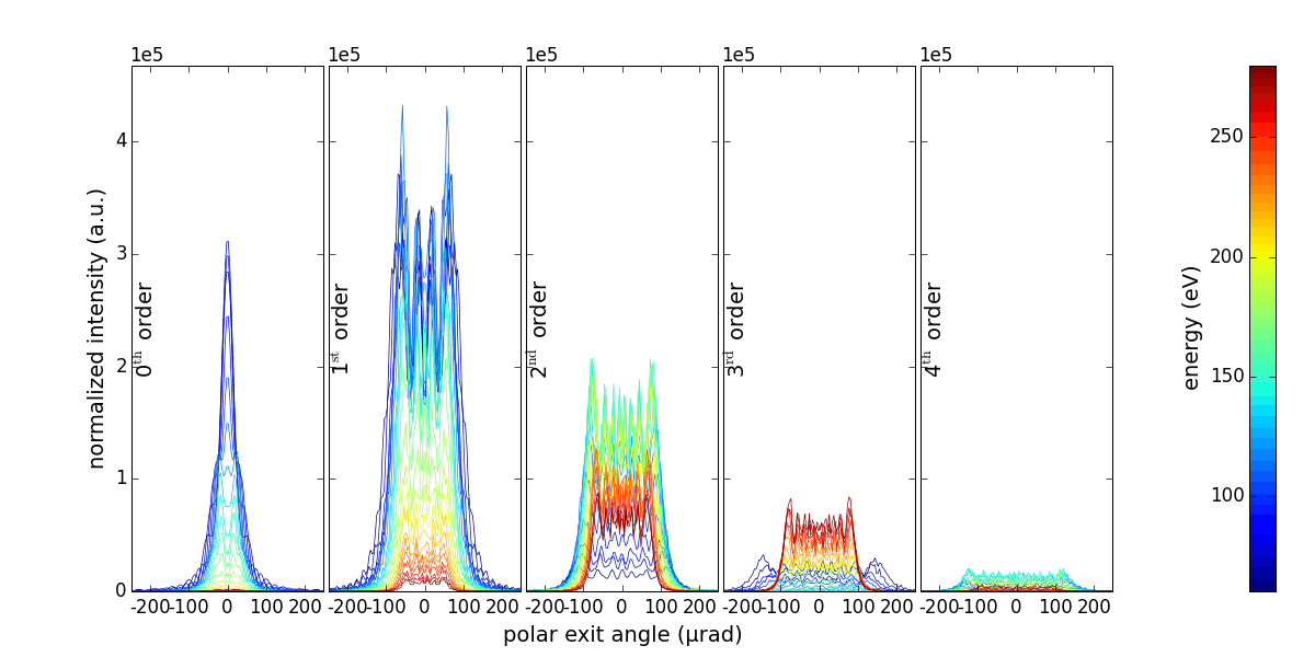
The diffraction orders are shown below as transverse images and meridional (“polar exit angle”) and sagittal (“azimuthal exit angle”) cuts. Notice that the diffraction orders are positioned on the screen “by themselves”, i. e. with only the use of the Kirchhoff diffraction integral. Also before it was possible to work with grating diffraction orders in xrt within the geometrical ray tracing approach. In that approach the rays were deflected according to the grating equation. Here, in wave propagation, the grating equation was only used to position the screen.

Notice that in contrast to the conventional grating theories (also used in REFLEC), the diffraction orders here have the sagittal dimension. And that dimension has diffraction fringes and a variable width, too!

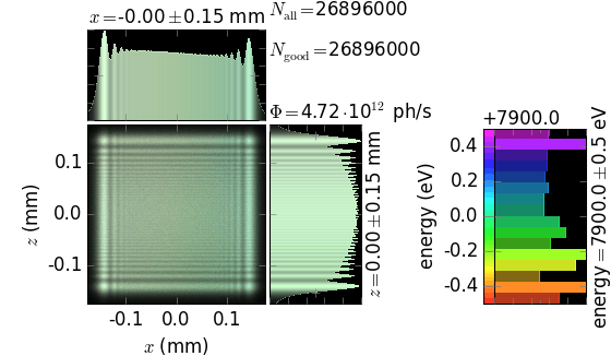
The resulting efficiency was obtained as ratio of the flux into the given order over the incoming flux. The incoming radiation was considered as uniform, parallel and fully coherent.

For the LEG (Low Energy Grating, see its properties in the figure below), the efficiency curves are pretty similar to those by REFLEC. The main difference is the low-energy part. Our 1st order does not decrease so rapidly. If we consider not the 2D exit angle but only the central azimuthal cut, the resulted low-energy efficiencies are very similar to that of REFLEC (not shown). Ref. [Boots] also provides experimental measurements which also have a rapid low-energy decrease. It seems that the detector had a pinhole that might cut the beam at low energies as the diffracted beam becomes wider there (see the transverse pictures above), which may explain lower measured efficiency.

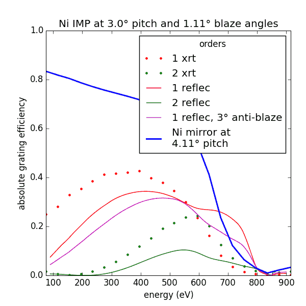
For the IMP grating (“impurity”, see its properties in the figure below), the difference is bigger.

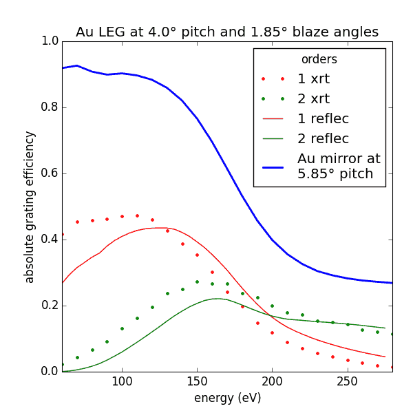
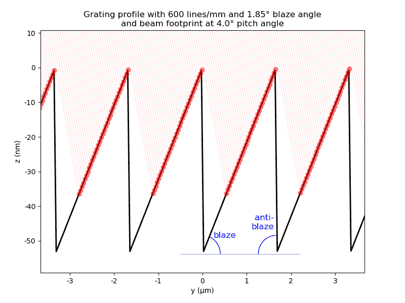
We believe that REFLEC is essentially wrong at high energies. If we mentally translate the working terraces of a blazed grating to form a continuous plane, we get a mirror at the pitch + blaze angle. By energy conservation, the overall grating efficiency (the sum into all orders) cannot be higher than the reflectivity of such a mirror. The REFLEC curves can violate this limit even for a single order, compare with the blue curve in the figure above. The reason for such behavior seems to be the artificially shadowless illumination by the incoming wave. Indeed, REFLEC assumes the complete saw profile to work in the diffraction, whereas the back side and a portion of the front side behind it stay in the shadow. We compare the two gratings shown below, one is with 90 degree anti-blaze angle and the other is with pitch as anti-blaze angle.

REFLEC gives different efficiencies for these two cases (see above) whereas xrt cannot distinguish them. We tried to artificially remove the shadows by making the surface “emit” a coherent wave. The result was an increase in the high-energy efficiency, similarly to the REFLEC’s behaviour.

The factors which definitely will affect the efficiency are (1) restricted coherence radius and (2) roughness. Both will be added into this example in a later release of xrt.

We are open for further discussion on the above results with interested scientists.

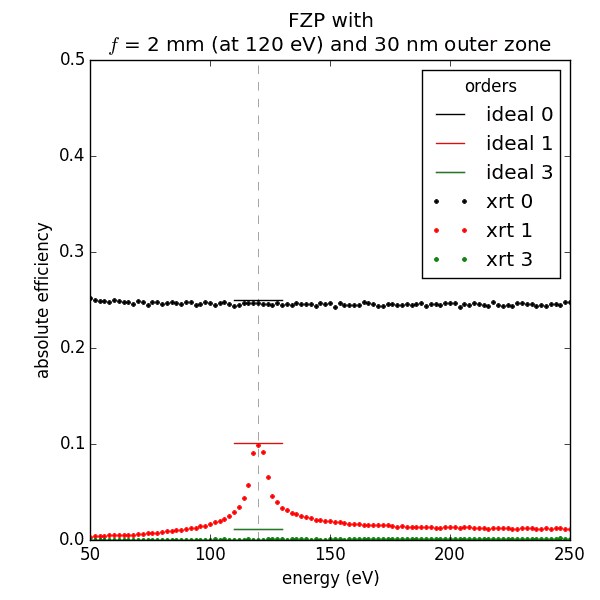
Diffraction from FZP

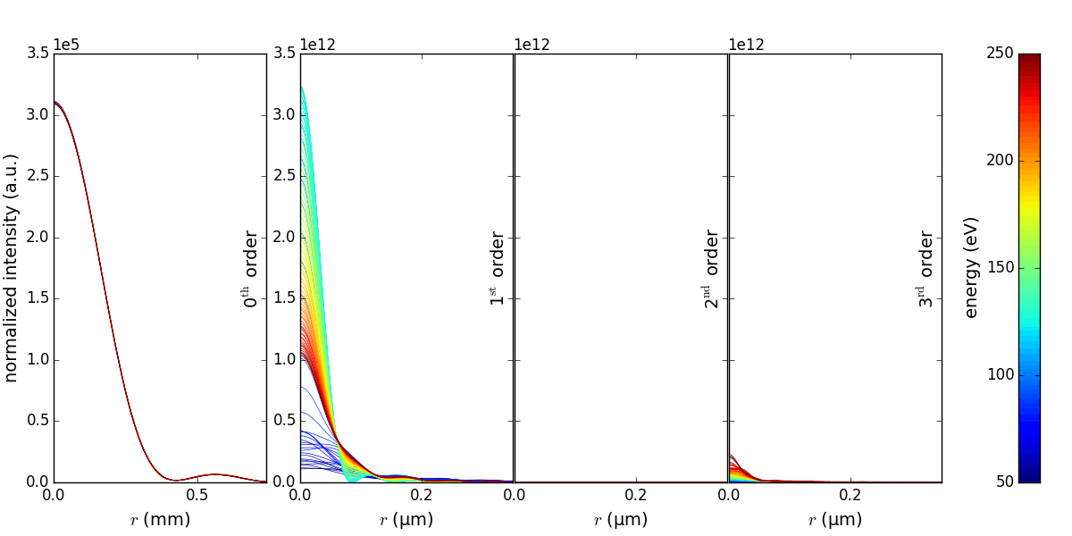
This examples demonstrates diffraction from a Fresnel Zone Plate with variously thick outer zone and at variable energy. The radial intensity distribution is shown in the figure below for a 70-nm-outer-zone FZP. Notice that the 2nd order was also calculated and together with other even orders indeed results in vanishing intensity.

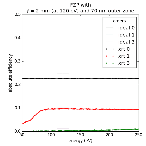
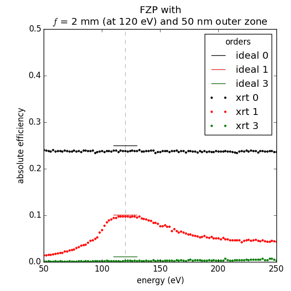
The energy dependence of efficiency for 3 different FZPs is shown below. The horizontal bars mark the expected \(1/m^2\pi^2\) levels for odd orders and 25% transmission for the 0th order. Watch how a zone plate becomes a band pass filter as the outer zone size approaches the wavelength, here ~10 nm.

SoftiMAX at MAX IV

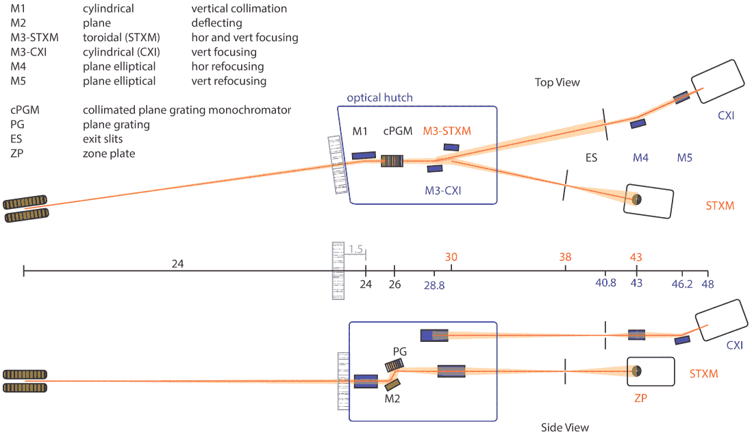
The images below are produced by scripts in \examples\withRaycing\14_SoftiMAX.

The beamline will have two branches: - STXM (Scanning Transmission X-ray Microscopy) and - CXI (Coherent X-ray Imaging),

see the scheme provided by K. Thånell.

STXM branch

Rays vs. hybrid

The propagation through the first optical elements – from undulator to front end (FE) slit, to M1, to M2 and to plane grating (PG) – is done with rays:

FE	M1	M2	PG

Starting from PG – to M3, to exit slit, to Fresnel zone plate (FZP) and to variously positioned sample screen – the propagation is done by rays or waves, as compared below. Despite the M3 footprint looks not perfect (not black at periphery), the field at normal surfaces (exit slit, FZP (not shown) and sample screen) is of perfect quality. At the best focus, rays and waves result in a similar image. Notice a micron-sized depth of focus.

	rays	wave
M3
exit slit
sample

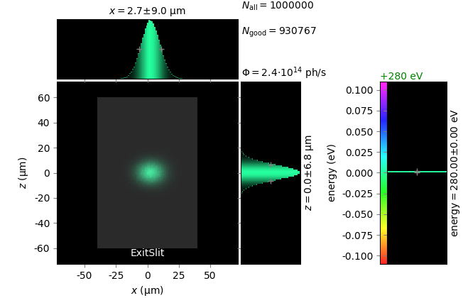
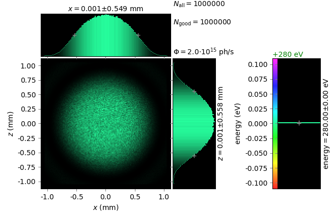
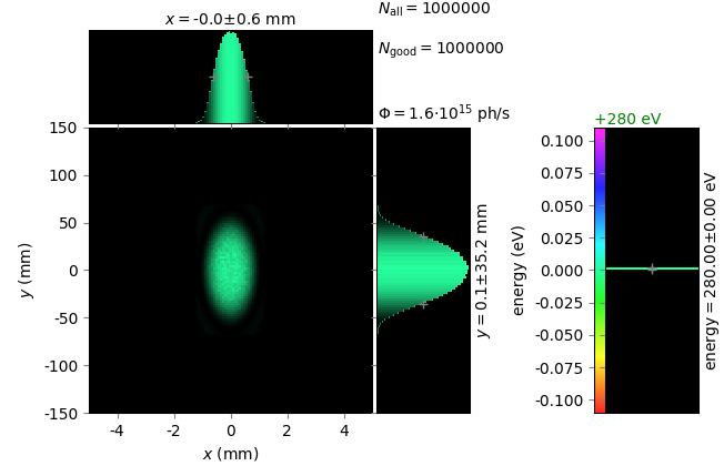
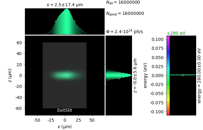
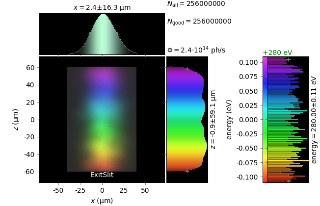
Influence of emittance

Non-zero emittance radiation is treated in xrt by incoherent addition of single electron intensities. The single electron (filament) fields are considered as fully coherent and are resulted from filament trajectories (one per repeat) that attain positional and angular shifts within the given emittance distribution. The following images are calculated for the exit slit and the focus screen for zero and non-zero emittance (for MAX IV 3 GeV ring: ε_x=263 pm·rad, β_x=9 m, ε_z=8 pm·rad, β_z=2 m). At the real emittance, the horizontal focal size increases by ~75%. A finite energy band, as determined by vertical size of the exit slit, results in somewhat bigger broadening due to a chromatic dependence of the focal length.

	0 emittance	real emittance	real emittance, finite energy band
exit slit
sample

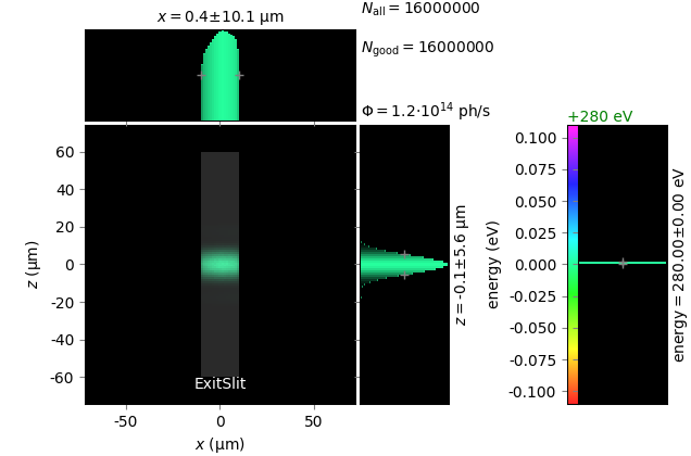
Correction of emittance effects

The increased focal size can be amended by closing the exit slit. With flux loss of about 2/3, the focal size is almost restored.

	80 µm exit slit	20 µm exit slit
exit slit
sample

Coherence signatures

The beam improvement can also be viewed via the coherence properties by the four available methods (see Coherence signatures). As the horizontal exit slit becomes smaller, one can observe the increase of the coherent fraction ζ and the increase of the primary (coherent) mode weight. The width of degree of coherence (DoC) relative to the width of the intensity distribution determines the coherent beam fraction. Both widths vary with varying screen position around the focal point such that their ratio is not invariant, so that the coherent fraction also varies, which is counter-intuitive. An important advantage of the eigen-mode or PCA methods is a simple definition of the coherent fraction as the eigenvalue of the zeroth mode (component); this eigenvalue appears to be invariant around the focal point, see below. Note that the methods 2 and 3 give equal results. The method 4 that gives the degree of transverse coherence (DoTC) is also invariant around the focal point, see DoTC values on the pictures of Principal Components.

	80 µm exit slit	20 µm exit slit
method 1
method 2
method 3, method 4b

CXI branch

2D vs 1D

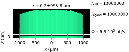
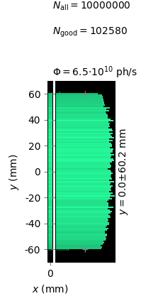
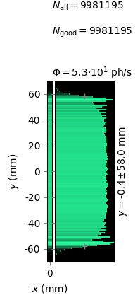
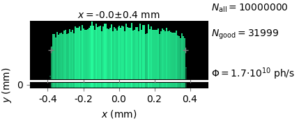
Although the sample screen images are of good quality (the dark field is almost black), the mirror footprints may be noisy and not well convergent in the periphery. Compare the M3 footprint with that in the previous section (STXM branch) where the difference is in the mirror area and thus in the sample density. The used 10⁶ wave samples (i.e. 10¹² possible paths) are not enough for the slightly enlarged area in the present example. The propagation is therefore performed in separated horizontal and vertical directions, which dramatically improves the quality of the footprints. Disadvantages of the cuts are losses in visual representation and incorrect evaluation of the flux.

	2D	1D horizontal cut	1D vertical cut
M3 footprint
sample screen

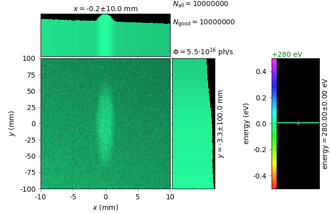
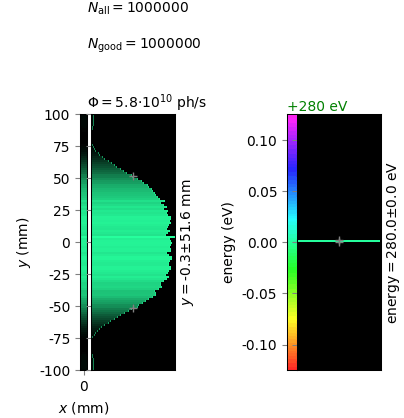
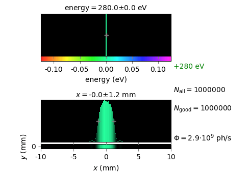
Flat screen vs normal-to-k screen (wave front)

The following images demonstrate the correctness of the directional Kirchhoff-like integral (see Sequential propagation). Five diffraction integrals are calculated on flat screens around the focus position: for two polarizations and for three directional components. The latter ones define the wave fronts at every flat screen position; these wave fronts are further used as new curved screens. The calculated diffraction fields on these curved screens have narrow phase distributions, as shown by the color histograms, which is indeed expected for a wave front by its definition. In contrast, the flat screens at the same positions have rapid phase variation over several Fresnel zones.

Note

In the process of wave propagation, wave fronts – surfaces of constant phase – are not used in any way. We therefore call it “wave propagation”, not “wave front propagation” as frequently called by others. The wave fronts in this example were calculated to solely demonstrate the correctness of the local propagation directions after having calculated the diffracted field.

flat screen	curved screen (wave front)

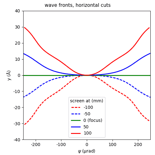
The curvature of the calculated wave fronts varies across the focus position. The wave fronts become more flat as one approaches the focus, see the figure below. This is in contrast to ray propagation, where the angular ray distribution is invariant at any position between two optical elements.

Rays, waves and hybrid

The following images are horizontal cuts at the footprints and sample screens calculated by

• rays,
• rays + waves hybrid (rays up to PG and wave from PG) and
• purely by waves.

	rays	hybrid	waves
front end slit		same as rays
footprint on M1		same as rays
footprint on M2		same as rays
footprint on PG		same as rays
footprint on M3
exit slit
footprint on M4
footprint on M5
sample screen

Coherence signatures

This section demonstrates the methods 1 and 3 from Coherence signatures. Notice again the difficulty in determining the width of DoC owing to its complex shape (at real emittance) or the restricted field of view (the 0 emittance case). In contrast, the eigen mode analysis yields an almost invariant well defined coherent fraction.

	0 emittance	real emittance
method 1
method 3

Defocusing by a distorted mirror

The images below are produced by \examples\withRaycing\13_Warping\warp.py.

This example has two objectives:

1. to demonstrate how one can add a functional or measured figure error to an ideal optical element and
2. to study the influence of various figure errors onto image non-uniformity in focused and defocused cases. The study will be done in ray tracing and wave propagation, the latter being calculated in partial coherence with the actual emittance of the MAX IV 3 GeV ring.

Here, a toroidal mirror focuses an undulator source in 1:1 magnification. The sagittal radius of the torus was determined for p = q = 25 m and pitch = 4 mrad. Defocusing in horizontal is done by going to a smaller pitch angle, here 2.2 mrad, and in vertical by unbending the meridional figure.

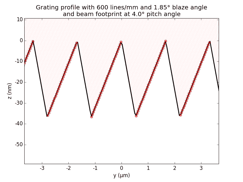
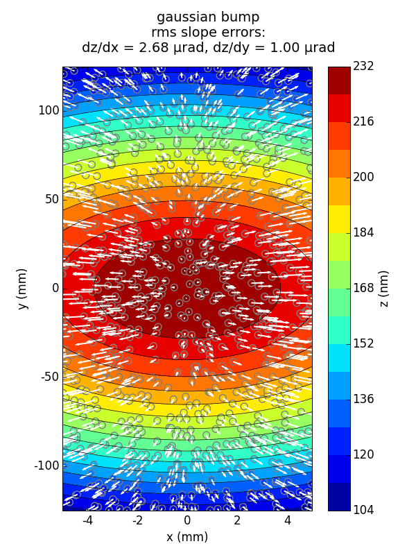
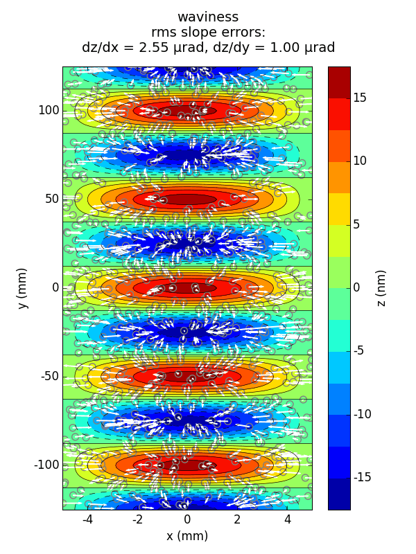
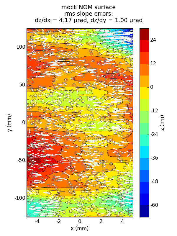
Three distorted surfaces are of Gaussian, waviness and as measured shapes, see below. They were normalized such that the meridional slope error be 1 µrad rms. The surfaces are determined on a 2D mesh. Interpolation splines for the height and the normal vector are found at the time of mirror instantiation and used in two special methods: local_z_distorted and local_n_distorted, see Section Distorted surfaces. If the distorted shape is known analytically, as for waviness, the two methods may directly invoke the corresponding functions without interpolation. The scattered circles in the figures are random samples where the height is calculated by interpolation (cf. the color (height) of the circles with the color of the surface) together with the interpolated normals (white arrows as projected onto the xy plane).

Gaussian	waviness	mock NOM measurement

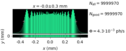
Defocused images reveal horizontal stripes seen both by ray tracing and wave propagation. Notice that wave propagation ‘sees’ less distortion in the best focusing case.

	ray tracing	wave propagation
ideal
Gaussian
waviness
mock NOM