Gallery of plots and scripts 2. X-ray optics

Beamline optics

The images below are produced by the scripts in \examples\withRaycing\02_Balder_BL\. The examples show the scans of various optical elements at Balder@MaxIV beamline. The source is a multipole conventional wiggler.

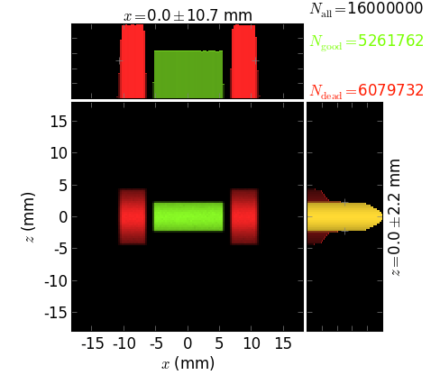
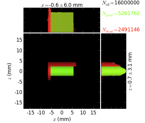
Diamond filter of varying thickness

Shown are i) intensity downstream of the filter and its energy spectrum and ii) absorbed power in the filter with its energy spectrum and power density isolines at 85% and 95% of the maximum.

White-beam collimating mirror at varying pitch angle

	bare Si	Ir coating
flux downstream of the mirror with its energy spectrum
absorbed power in the mirror with its energy spectrum and power density isolines at 90% of the maximum

Bending of collimating mirror

Shown are i) image downstream of the DCM and ii) image at the sample.

Bending of focusing mirror

Shown is the image at the sample position.

Both mirrors (collimating + focusing) at varying pitch angle

The sagittal radius of the focusing toroid mirror is optimal at 2 mrad pitch angle.

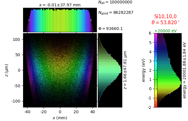
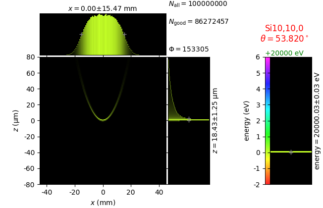
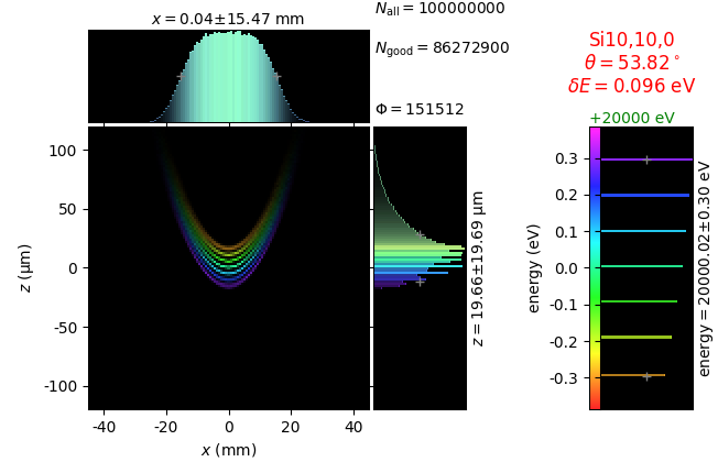
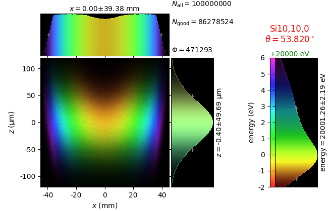
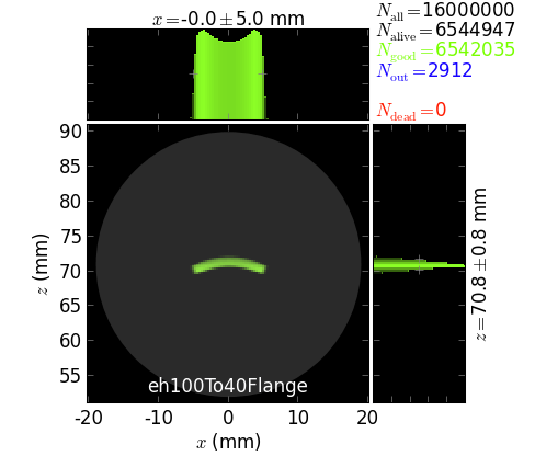
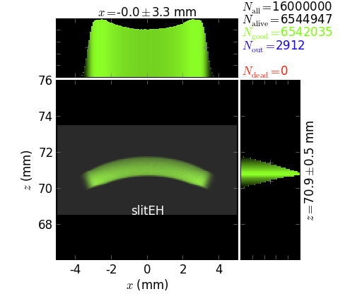
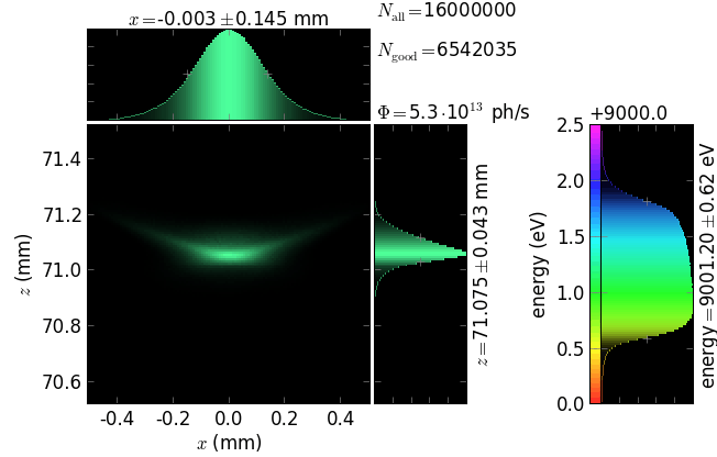
Scanning of Double Crystal Monochromator

Scanning of Double Multilayer Monochromator

This example shows a scan of a double multilayer monochromator – analog of a double crystal monochromator. On the left is the footprint on the 1st multilayer. On the right is a transversal image of the exit beam. The two multilayers are equal and have 40 pairs of 27-Å-thick silicon on 18-Å-thick tungsten layers on top of a silicon substrate.

Laue Monochromator

Bending of a single crystal Laue Monochromator

Files in \examples\withRaycing\03_LaueMono

This example shows the reflectivity of a bent 200-µm-thick Si111 Laue crystal at various bending radii and energies. Watch how the band width is growing and the flux is lowering in going to smaller radii.

E = 9 keV	E = 16 keV	E = 25 keV	E = 36 keV

Double bent-crystal Laue monochromator (beam cleaner)

This example shows the beam images and rocking curves of a bent 200-µm-thick Si111 double Laue crystal monochromator (similar to the beam cleaner [Karanfil2004]) at various bending radii and energies.

[Karanfil2004]

C. Karanfil, D. Chapman, C. U. Segre and G. Bunker, A device for selecting and rejecting X-ray harmonics in synchrotron radiation beams, J. Synchrotron Rad. 11 (2004) 393-8.

Beam images at various detuning angles of the second crystal, R = 25 m, E ~ 9 keV. Watch how the energy band becomes split and the flux goes down in going away from the parallel positioning (dθ = 0).

Flux vs. detuning angle of the second crystal (rocking curves)

E = 9 keV	E = 16 keV	E = 25 keV	E = 36 keV

Compound Refractive Lenses

Files in \examples\withRaycing\04_Lenses

This example demonstrates refraction in x-ray regime. Locus that refracts a collimated beam into a point focus is a paraboloid. The focal distance of such a vacuum-to-solid interface is, as in the usual optics, 2p/δ where p is the focal parameter of the lens paraboloid and δ = 1 - Re(n), n is the refractive index [snigirev]. As for the usual lenses, the diopters of several consecutive lenses are summed up to give the total diopter: \(\frac{1}{f} = \frac{1}{f_1} + \frac{1}{f_2} + \ldots\).

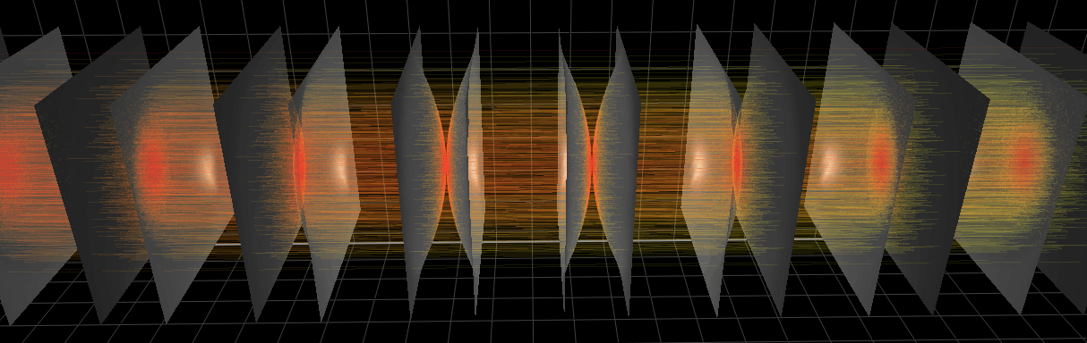
This example considers focusing of collimated x-rays of 9 keV at a distance q = 5 m from the lenses. The lenses are double-sided paraboloids (then f = p/δ) with p = 1 mm and zero spacing between the apices of the paraboloids. The thickness of each lens is 2 mm. Their number is an integer number N = round(p/qδ).

The following images demonstrate the focusing along the optical axis close to the nominal focal position for Be and Al CRL’s. The real focal position deviates from the nominal one, where dq = 0, due to the rounding of p/qδ:

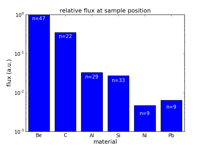
This graph shows the relative flux in the focused beam at 9 keV after the given number of double-sided lenses which give approximately equal focal distance of q = 5 m. As seen, low absorbing materials are preferred:

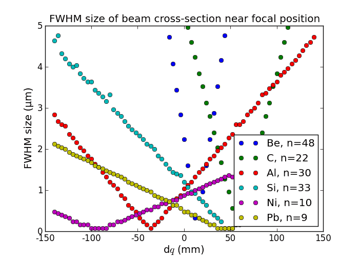
This graph shows the depth of focus as a function of the on-axis coordinate around the nominal focal position. For heavy materials the depth of focus is larger due to the higher absorption of the peripherical rays of the incoming beam. Such lenses act effectively also as apertures thus reducing the focal spot at the expense of flux:

[snigirev]

A. Snigirev, V. Kohn, I. Snigireva, A. Souvorov, and B. Lengeler, Focusing High-Energy X Rays by Compound Refractive Lenses, Applied Optics 37 (1998), 653-62.

Quarter wave plates

Files in \examples\withRaycing\05_QWP

Collimated beam, Bragg transmission case

This example shows the polarization properties of a collimated linearly polarized beam passed through a diamond plate at various departure from the nominal Bragg angle. The polarization plate is put at 45º to the diffraction plane. Notice that the phase difference between the s- and p-polarized components was calculated here not in the 1-field approximation as elsewhere [Malgrange] that has a pole at \(\Delta\theta=0\) but in the general 2-field approximation, see materials.

[Malgrange]

C. Giles, C. Malgrange, J. Goulon, F. de Bergevin, C. Vettier, E. Dartyge, A. Fontaine, C. Giorgetti and S. Pizzini, J. Appl. Cryst. 27 (1994) 232; C. Giles, C. Vettier, F. de Bergevin, C. Malgrange, G. Grübel, and F. Grossi, Rev. Sci. Instrum. 66 (1995) 1518; J. Goulon, C. Malgrange, C. Giles, C. Neumann, A. Rogalev, E. Moguiline, F. De Bergevin and C. Vettier, J. Synchrotron Rad. 3 (1996) 272.

Beam images after the QWP with color axis as 1) energy, 2) circular polarization rate, 3) phase shift between s- and p-components and 4) ratio of axes of the polarization ellipse. Watch how the circular polarization rate becomes close to 1 or -1 at certain departure angles; here, between 16 and 32 arcsec (plus or minus). At the same time also the ratio of axes of the polarization ellipse becomes close to 1 or -1 and with narrow distribution.

E ~ 9 keV, crystal thickness = 200 µm.

Collimated beam, Laue transmission case

Same as in the revious subsection but for the Laue case. The thickness of the crystal was selected as to give the path length similar to that in the Bragg case.

E ~ 9 keV, crystal thickness = 500 µm.

Convergent beam, Laue transmission case

In this example the beam is focused by a toroidal mirror. Due to the large angular variation in the beam (3 mrad at the position of the QWP), the resulting circular polarization rate is low. The initial polarization is horizontal and the diffraction plane of the QWP is turned by 45º from vertical.

E ~ 9 keV, crystal thickness = 500 µm.

Convergent beam, bent-Laue transmission case

One way to improve the low circular polarization rate in a divergent or convergent beam is to aperture it, with the obvious disadvantage of lowering the beam flux. Another, less obvious, way is to bend the crystal with the radius equal to the distance from the sample (focal point) to the QWP. In this particular example the Laue case is considered. The bending is done cylindrically in the diffraction plane which is at 45º to the initial polarization plane (horizontal). Watch the circular polarization rate at \(\pm\) 32 arcsec departure angle.

E ~ 9 keV, crystal thickness = 500 µm.

Comparison of 1D-bent crystal analyzers

Files in /examples/withRaycing/06_AnalyzerBent1D

Rowland circle based analyzers

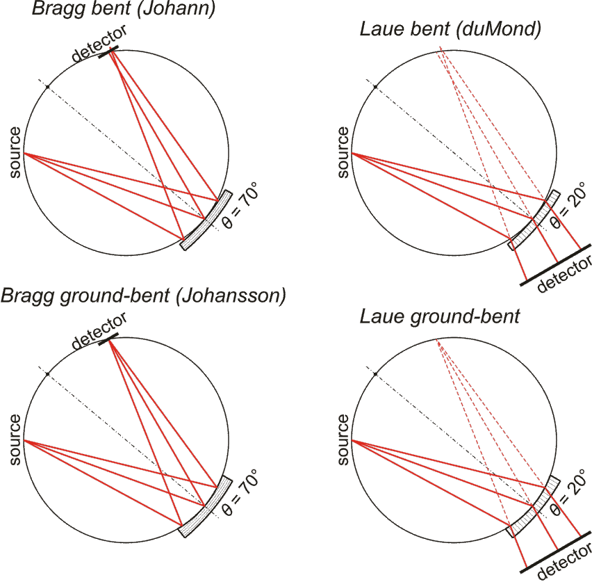
This study compares simply bent and ground-bent spectrometers utilizing Bragg and Laue analyzing crystals. The bending is cylindrical (one-dimensional).

Conditions:

Rowland circle diameter = 1 m, 70v × 200h µm² unpolarized fluorescence source, crystal size = 100meridional × 20saggittal mm².

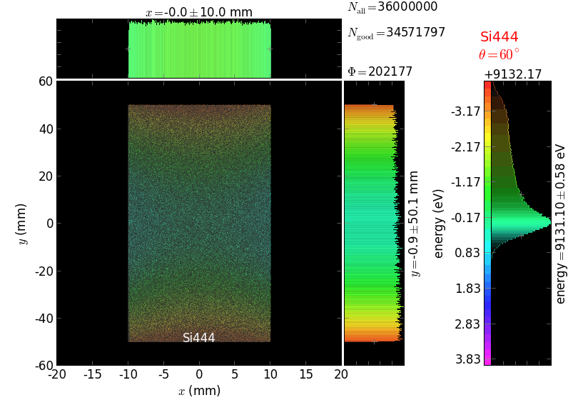
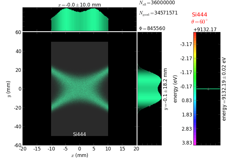
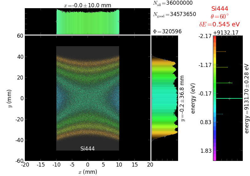
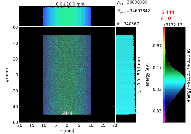
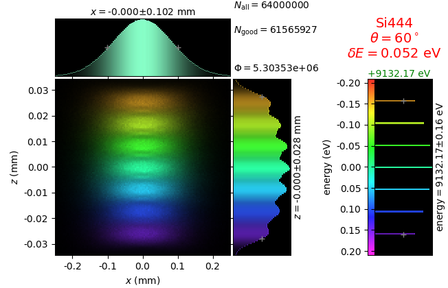
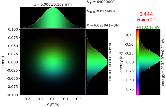
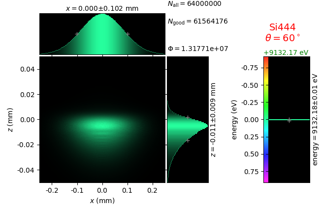
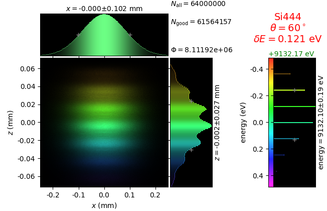
Energy resolution was calculated as described in the CDR of a diced Johansson-like spectrometer at Alba/CLÆSS beamline. This calculation requires two images: 1) of a flat energy distribution source and 2) of a monochromatic source. The images are dispersive in the diffraction plane, which can be used in practice with a position sensitive detector or with a slit scan in front of a bulk detector. From these two images energy resolution δE was calculated and then 3) a verifying image was ray-traced for a source of 7 energy lines evenly spaced with the found step δE. Such images are shown for the four crystal geometries at a particular Bragg angle:

geometry	flat source	line source	7 lines
Bragg simply bent
Bragg ground bent
Laue simply bent
Laue ground bent

The energy distribution over the crystal surface is hyperbolic for Bragg and ellipsoidal for Laue crystals. Therefore, Laue crystals have limited acceptance in the sagittal direction whereas Bragg crystals have the hyperbola branches even for large sagittal sizes. Notice the full crystal coverage in the meridional direction for the two ground-bent cases.

geometry	flat source	line source	7 lines
Bragg simply bent
Bragg ground bent
Laue simply bent
Laue ground bent

As a matter of principles checking, let us consider how the initially unpolarized beam becomes partially polarized after being diffracted by the crystal analyzer. As expected, the beam is fully polarized at 45° Bragg angle (Brewster angle in x-ray regime). CAxis here is degree of polarization:

Bragg	Laue

Comments

1. The ground-bent crystals are more efficient as the whole their surface works for a single energy, as opposed to simply bent crystals which have different parts reflecting the rays of different energies.

2. When the crystal is close to the source (small θ for Bragg and large θ for Laue spectrometers), the images are distorted, even for the ground-bent crystals.

3. The Bragg case requires small pixel size in the meridional direction (~10 µm for 1-m-diameter Rowland circle) for a good spatial resolution but can profit from its compactness. The Laue case requires a big detector of a size comparable to that of the crystal but the pixel size is not required to be small.

4. The comparison of energy resolution in Bragg and Laue cases is not strictly correct here. While the former case can use the small beam size at the detector for utilizing energy dispersive property of the spectrometer, the latter one has a big image at the detector which is restricted by the size of the crystal. The size of the ‘white’ beam image is therefore correct only for the crystal size selected here. The Laue case can still be used in energy dispersive regime if 2D image analysis is utilized. At the present conditions, the energy resolution of Bragg crystals is better than that of Laue crystals except at small Bragg angles and low diffraction orders.

5. The energy resolution in ground-bent cases is not always better than that in simply bent cases because of strongly curved images. If the sagittal size of the crystal is smaller or sagittal bending is used, the advantage of ground-bent crystals is clearly visible not only in terms of efficiency but also in terms of energy resolution.

Johansson analyzer with elastically deformed crystal

Example in /examples/withRaycing/06_AnalyzerBent1D/01B_BentTT.py

A Johansson 1D ground-bent analyzer is studied here by ray tracing with two ways of reflectivity calculations: for a perfect crystal and for an elastically deformed crystal by means of the Takagi-Taupin equations. For higher reflection indices, the deviation from perfect crystal reflectivity becomes increasingly pronounced. Notice here an increased flux value and decreased energy resolution for the latter case.

study	flat source	line source	7 lines
perfect crystal
deformed crystal (Takagi- Taupin)

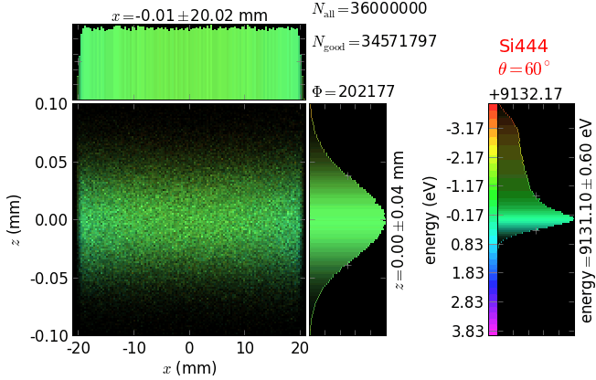
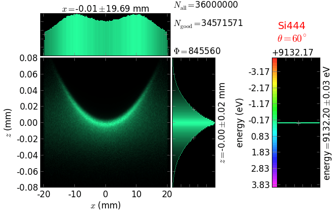
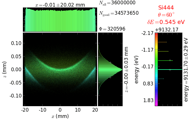
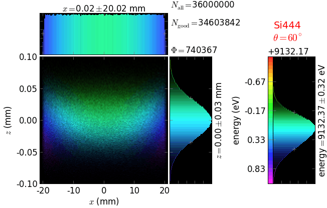
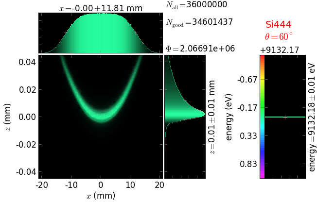
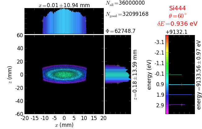
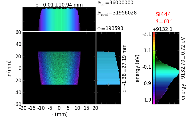
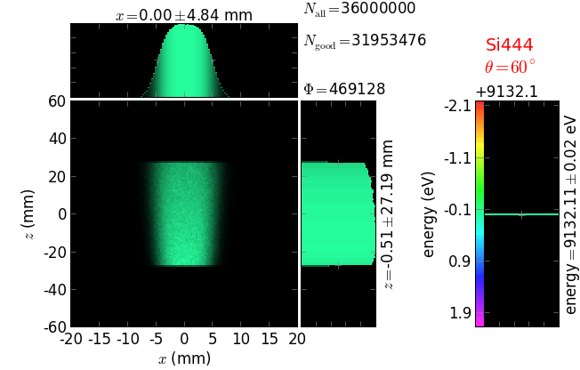
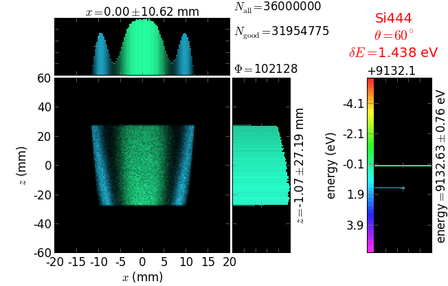
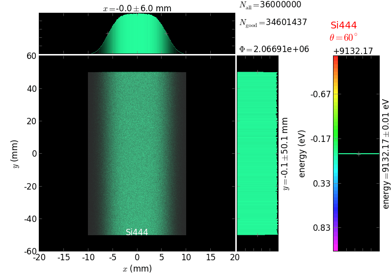
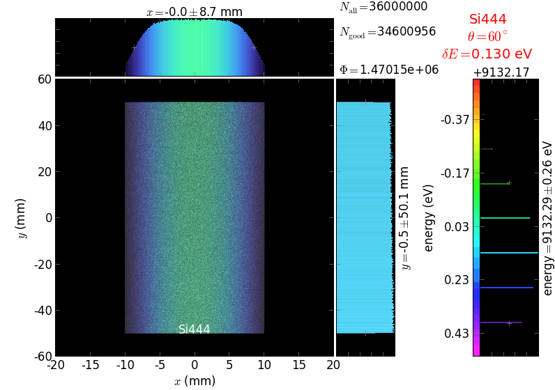
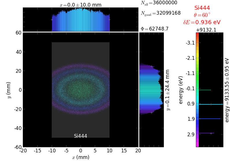
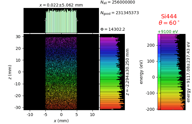
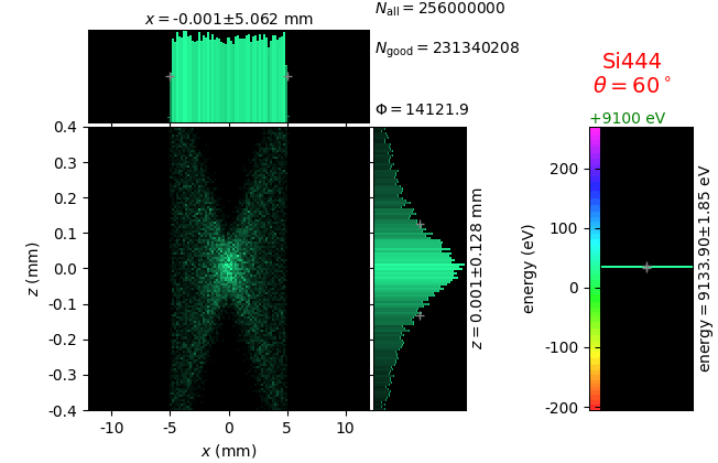
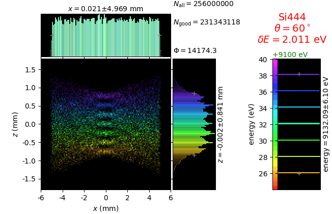
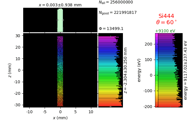
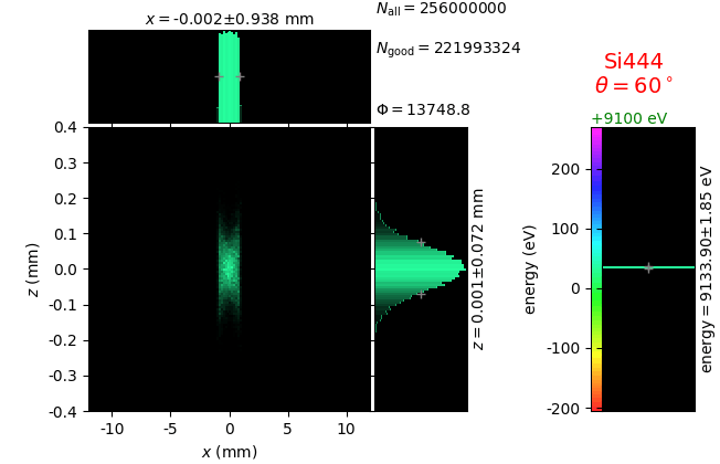
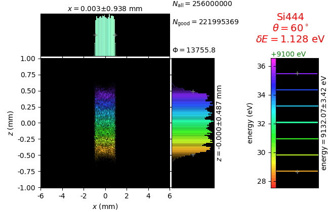
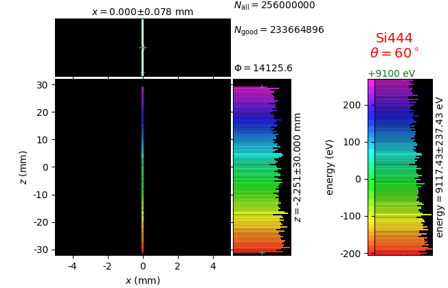
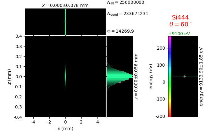
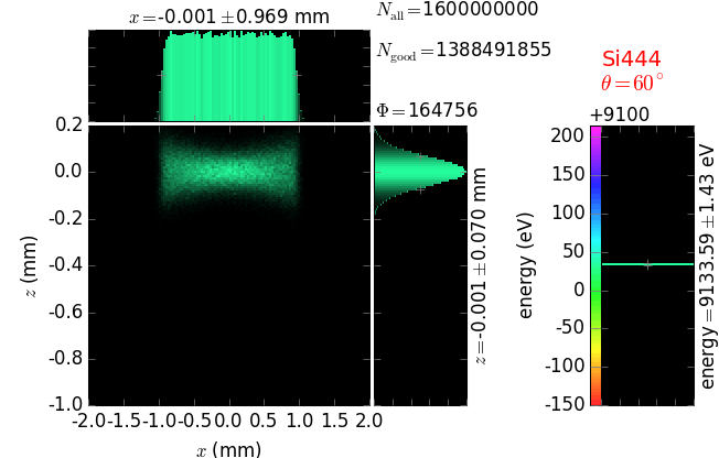
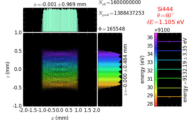
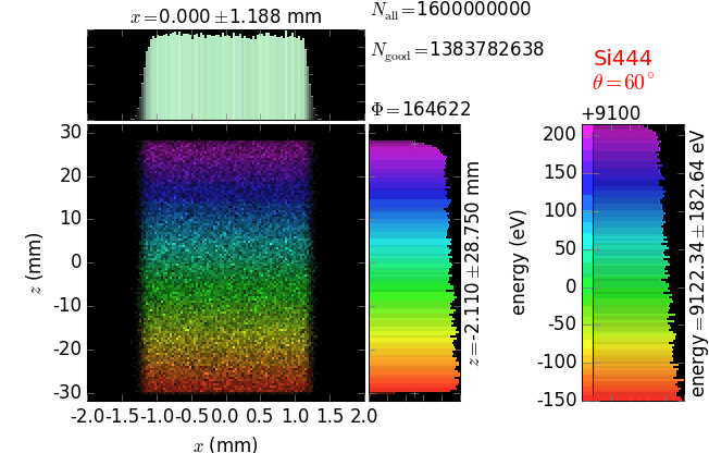
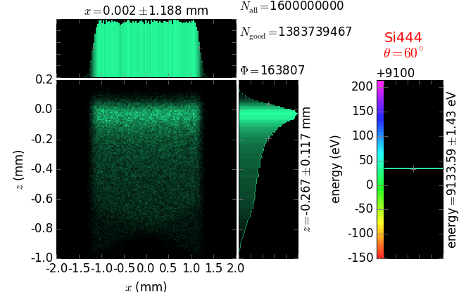
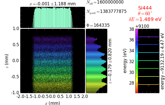
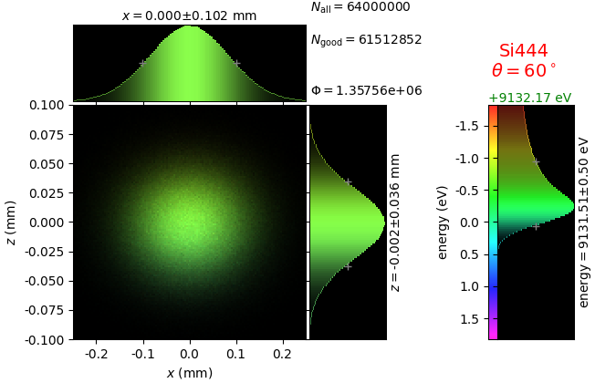
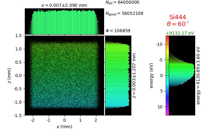
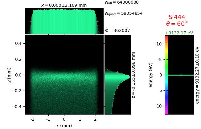
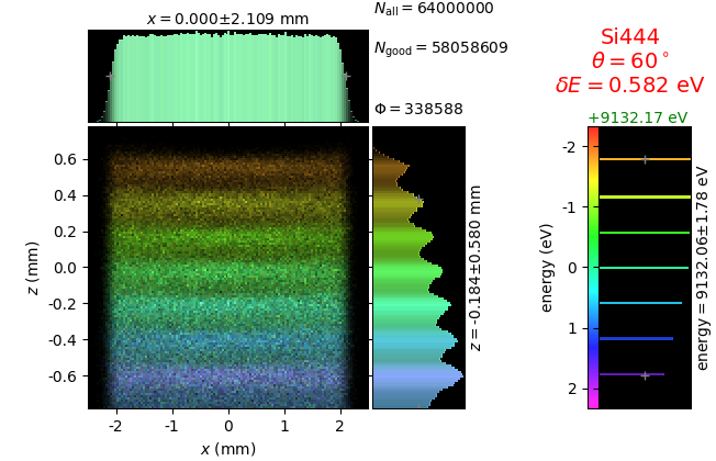
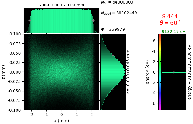
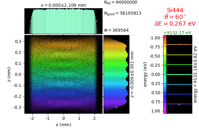
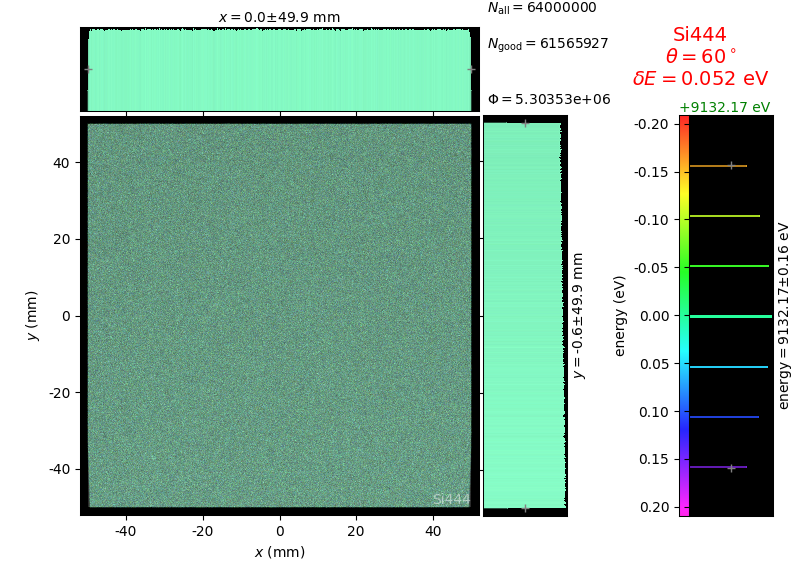
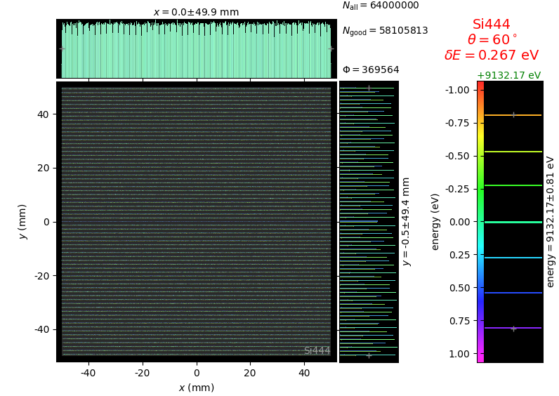
Von Hamos analyzer

A von Hamos spectrometer has axial symmetry around the axis connecting the source and the detector. The analyzing crystal is cylindrically bent with the radius equal to the crystal-to-axis distance. In this scheme, the emission escape direction depends on Bragg angle (energy). In practice, the spectrometer axis is adapted such that the escape direction is appropriate for a given sample setup. If the emission escape direction is kept fixed relatively to the sample, the mechanical model becomes more complex and includes three translations and two rotations. In the figure below, the crystal is sagittally curved around the source-detector line. The detector plane is perpendicular to the sketch. Left: the classical setup [vH] with 2 translations. Right: the setup with an invariant escape direction.

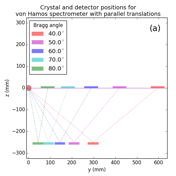
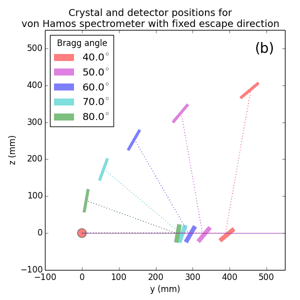
The geometrical parameters for the von Hamos spectrometer were taken from [vH_SLS]: a diced 100 (sagittal) × 50 (meridional) mm² Si(444) crystal is curved with Rs = 250 mm. The width of segmented facets was taken equal to 5 mm (as in [vH_SLS]) and 1 mm together with a continuously bent case. The crystal thickness = 100 µm.

[vH] (1,2)

L. von Hámos, Röntgenspektroskopie und Abbildung mittels gekrümmter Kristallreflektoren II. Beschreibung eines fokussierenden Spektrographen mit punktgetreuer Spaltabbildung, Annalen der Physik 411 (1934) 252-260

[vH_SLS] (1,2)

J. Szlachetko, M. Nachtegaal, E. de Boni, M. Willimann, O. Safonova, J. Sa, G. Smolentsev, M. Szlachetko, J. A. van Bokhoven, J.-Cl. Dousse, J. Hoszowska, Y. Kayser, P. Jagodzinski, A. Bergamaschi, B. Schmitt, C. David, and A. Lücke, A von Hamos x-ray spectrometer based on a segmented-type diffraction crystal for single-shot x-ray emission spectroscopy and time-resolved resonant inelastic x-ray scattering studies, Rev. Sci. Instrum. 83 (2012) 103105.

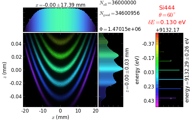
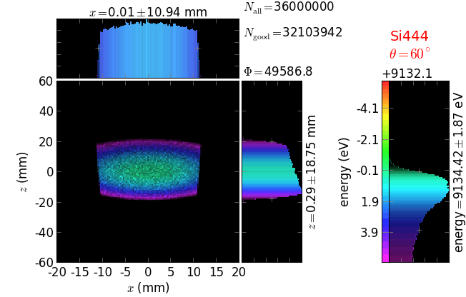
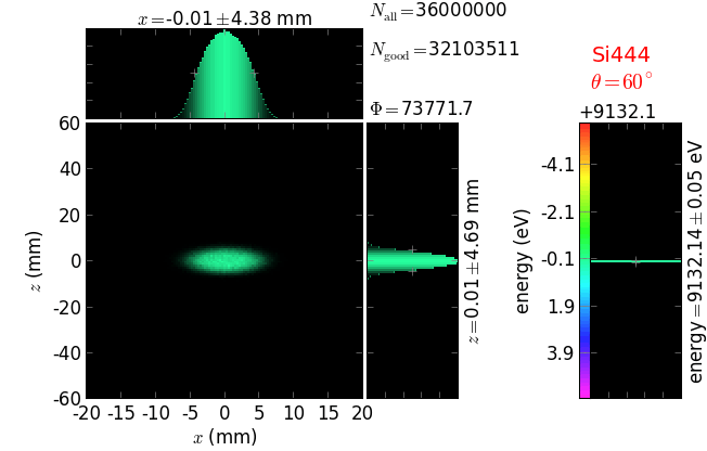
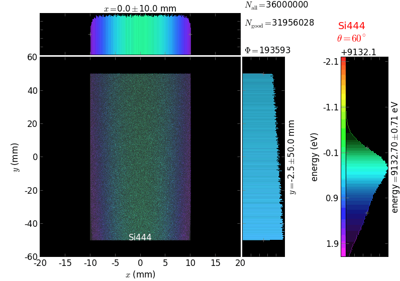
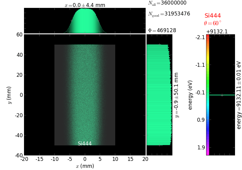
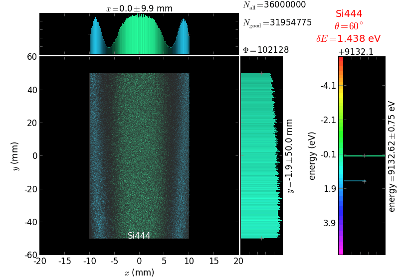
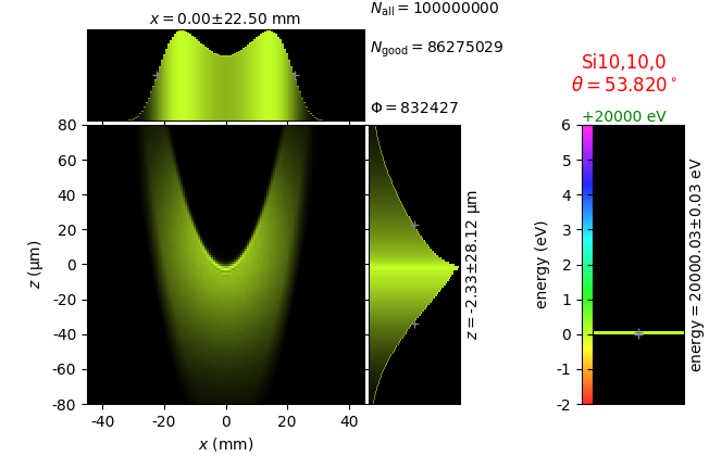
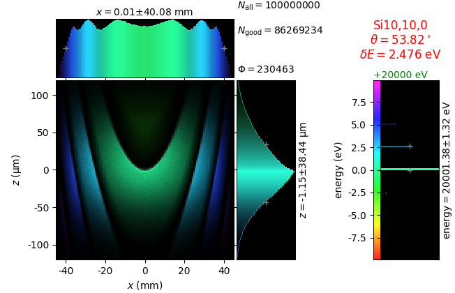
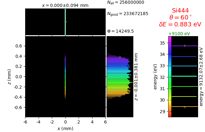
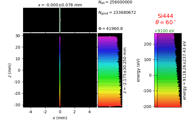
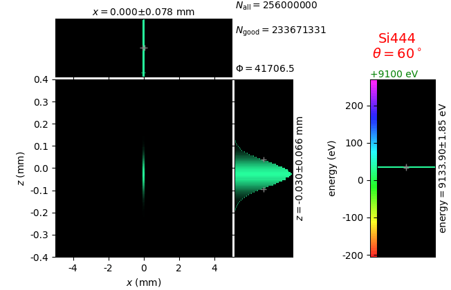
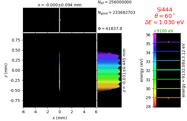
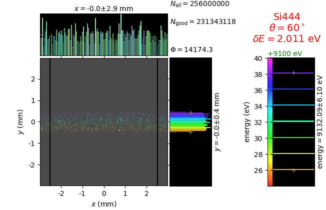
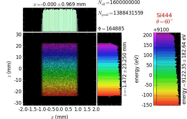
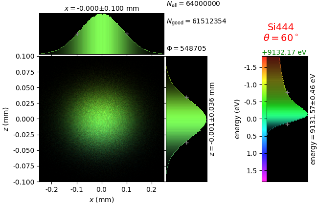
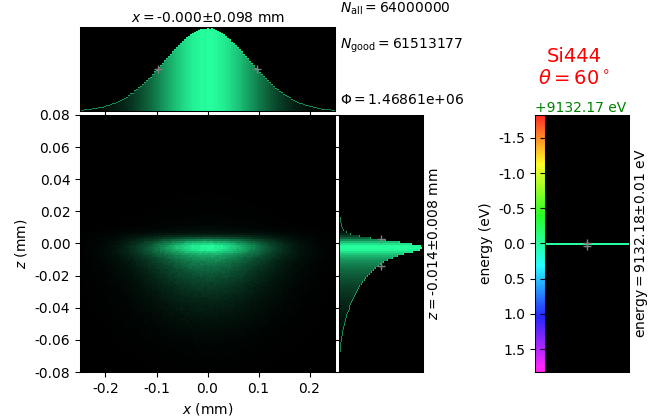
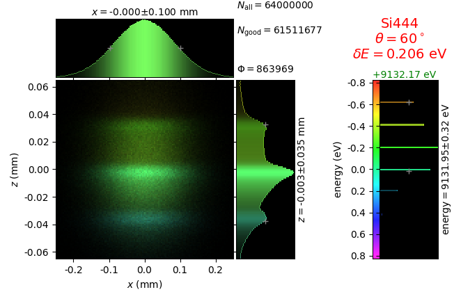
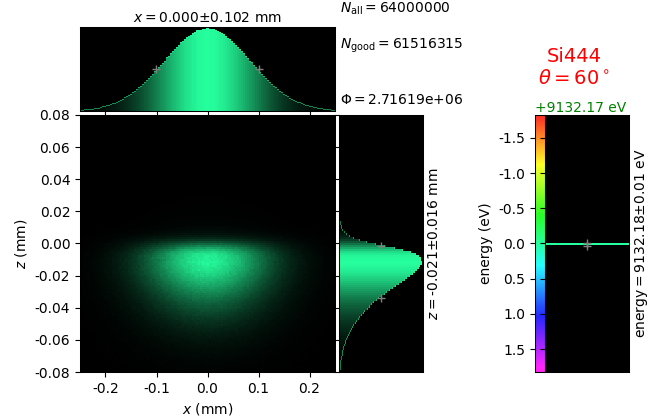
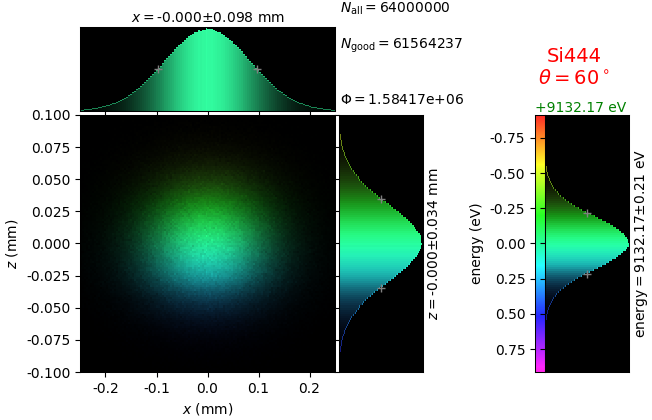
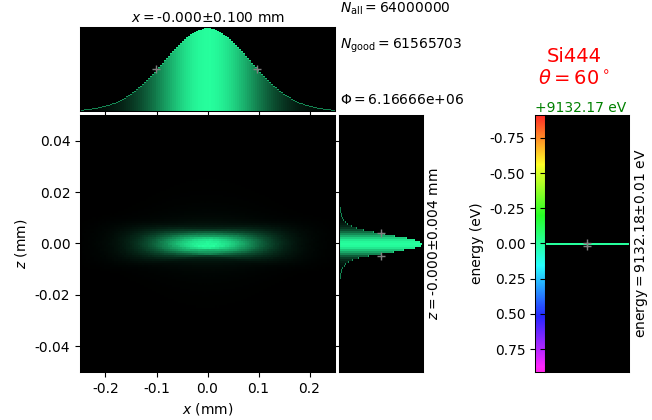
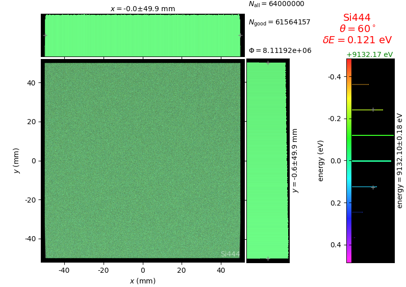
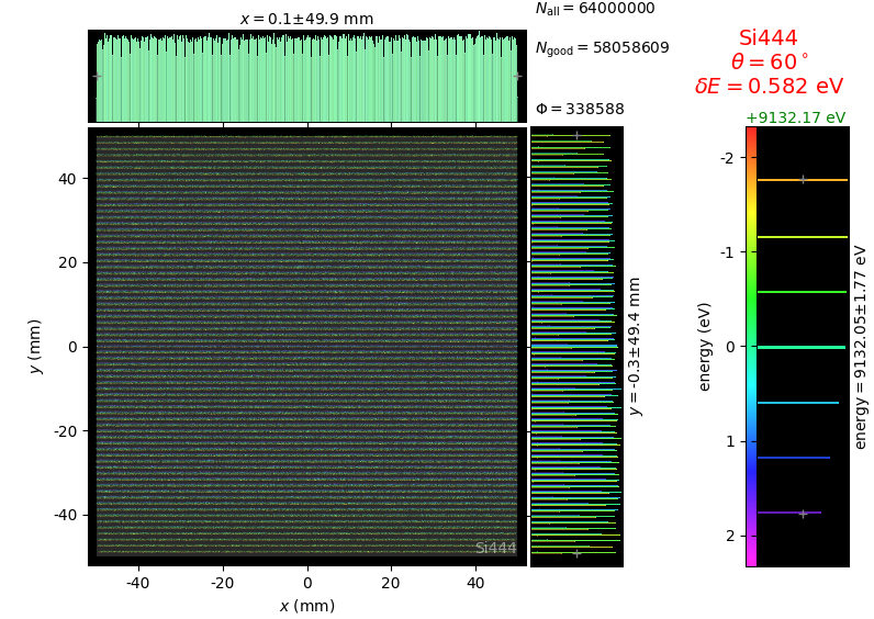
The calculation of energy resolution requires two detector images: 1) of a flat energy distribution source and 2) of a monochromatic source. From these two images, energy resolution δE was calculated and then 3) a verifying image was ray-traced for a source of 7 energy lines evenly spaced with the found step δE. Such images are shown for different dicing sizes at a particular Bragg angle. In addition to perfect crystal reflectivity calculations, elastically deformed crystal reflectivity was calculated by means of the Takagi-Taupin equations (labelled TT).

crystal	flat source	line source	7 lines
diced 5 mm
diced 1 mm
not diced
not diced TT

With the coloring by stripe (crystal facet) number, the image below explains why energy resolution is worse when stripes are wider and the crystal is sagittally larger. The peripheral stripes contribute to aberrations which increase the detector image.

crystal	line source colored by stripe number
diced 5 mm
diced 1 mm

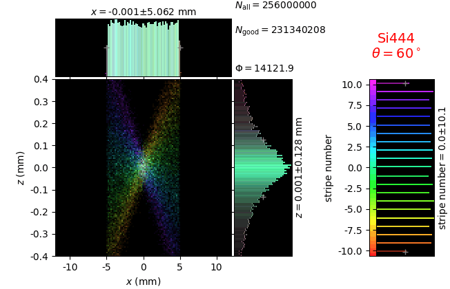
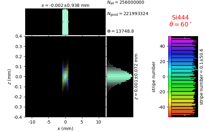
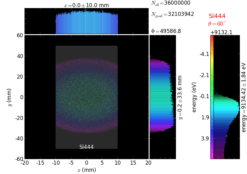
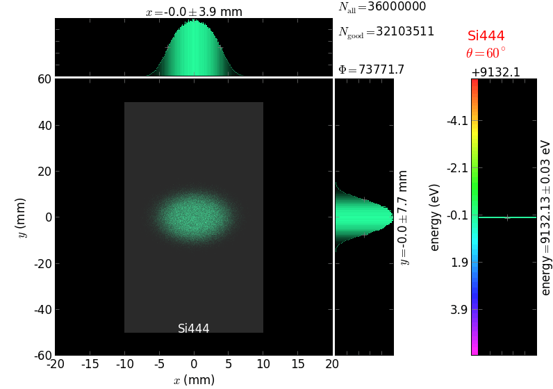
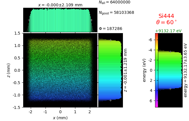
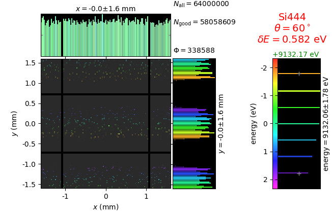
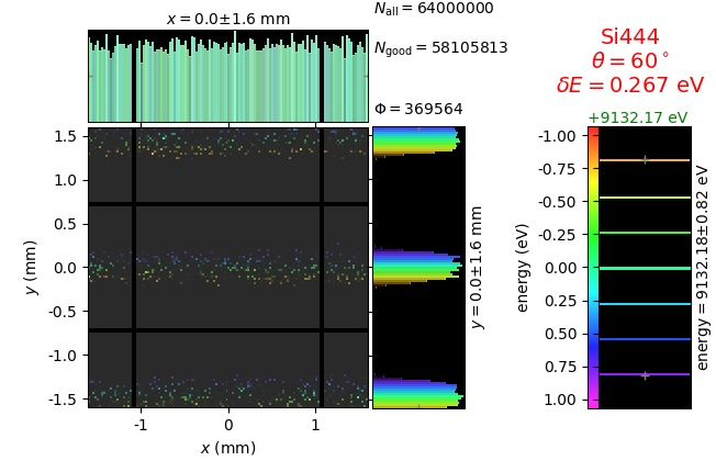
The efficiency of a von Hamos spectrometer is significantly lower as compared to Johann and Johansson crystals. The reason for the lower efficiency can be understood from the figure below, where the magnified footprint on the crystal is shown: only a narrow part of the crystal surface contributes to a given energy band. Here, in the 5-mm-stripe case a bandwidth of ~12 eV uses less than 1 mm of the crystal!

Comparison of Rowland circle based and von Hamos analyzers

An additional case was also included here: when a Johann crystal is rotated by 90⁰ around the sample-to-crystal line, it becomes a von Hamos crystal that has to be put at a correct distance corresponding to the 1 m sagittal radius. This case is labelled as “Johann as von Hamos”.

In comparing with a von Hamos spectrometer, one should realize its strongest advantage – inherent energy dispersive operation without a need for energy scan. This advantage is especially important for broad emission lines. Below, the comparison is made for two cases: (1) a narrow energy band (left figure), which is more interesting for valence band RIXS and which assumes a high resolution monochromator in the primary beam and (2) a wide energy band (right figure), which is more interesting for core state RIXS and normal fluorescence detection. The desired position on the charts is in the upper left corner. As seen in the figures, the efficiency of the von Hamos crystals (i) is independent of the energy band (equal for the left and right charts), which demonstrates truly energy-dispersive behavior of the crystals but (ii) is significantly lower as compared to the Johann and Johansson crystals. A way to increase efficiency is to place the crystal closer to the source, which obviously worsens energy resolution because of the increased angular source size. Inversely, if the crystal is put at a further distance, the energy resolution is improved (square symbols) but the efficiency is low because of a smaller solid angle collected. The left figure is with a narrow energy band equal to the 6-fold energy resolution. The right figure is with a wide energy band equal to 8·10 ^-4·E (approximate width of K β lines [Henke]).

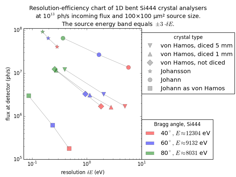
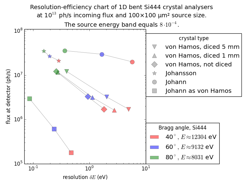
Finally, among the compared 1D-bent spectrometers the Johansson type is the best in the combination of good energy resolution and high efficiency. It is the only one that can function both as a high resolution spectrometer and a fluorescence detector. One should bear in mind, however, two very strong advantages of von Hamos spectrometers: (1) they do not need alignment – a crystal and a detector positioned approximately will most probably immediately work and (2) the image is inherently energy dispersive with a flat (energy independent) detector response. The low efficiency and mediocre energy resolution are a price for the commissioning-free energy dispersive operation. Rowland circle based spectrometers will always require good alignment, and among them only the Johansson-type spectrometer can be made energy dispersive with a flat detector response.

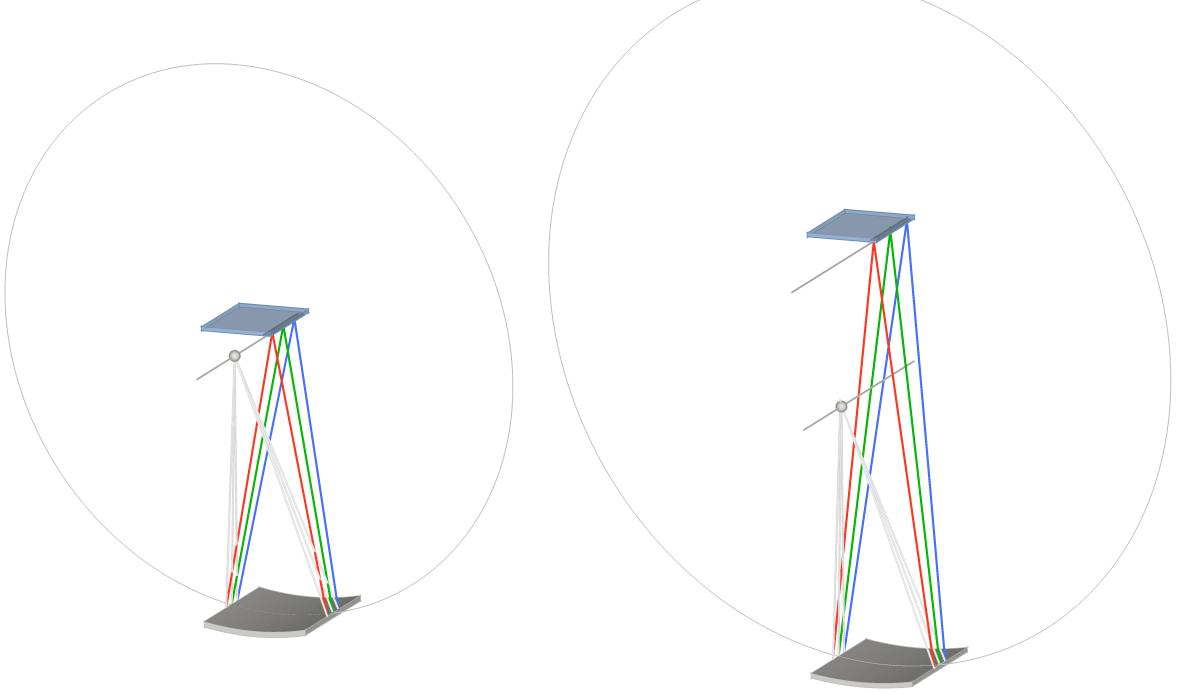
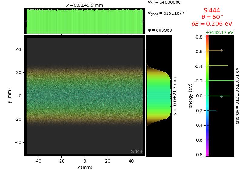
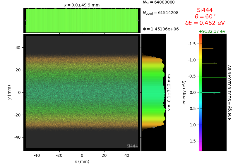
Circular and elliptical von Hamos analyzers

The axial symmetry of the classical von Hamos spectrometer [vH] results in a close detector-to-sample position at large Bragg angles. A single detector may find enough space there but when the spectrometer has several branches, the corresponding detectors come close to each other, which restricts both the space around the sample and the accessible Bragg angle range. A solution to this problem could be an increased magnification of the crystal from the classical 1:1. The axis of the circular cilynder is then split into two axes representing the two foci of an ellipsoid, see the scheme below. The lower axis holds the source (sample) and the upper one holds the detector. The crystal in the figure has the magnification 1:1 for the circular crystal (left part) and 1.5:1 for the elliptical one (right part).

The crystal is diced along the cylinder axis with 1 mm pitch. The difference in the circular and elliptical figures is shown below.

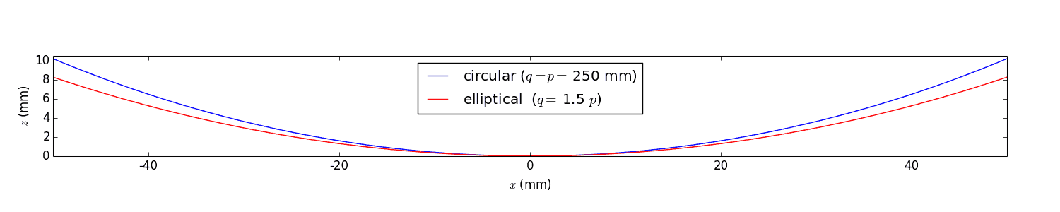
The elliptical figure results in some aberrations, as seen by the monochromatic images below, which worsens energy resolution.

crystal	flat source	line source	7 lines
bent as circular cylinder
bent as elliptical cylinder

Comparison of 2D-bent Bragg crystal analyzers

Files in \examples\withRaycing\07_AnalyzerBent2D

This study compares simply bent (Johann) and ground-bent (Johansson) analyzers in diced and non-diced versions. This time the bending is two-dimensional with the sagittal radius equal to the distance from the crystal to the source-detector line. Such bending gives a family of Rowland circles all going through the source and the detector.

The conditions are equal to those in the previous section. The crystal size is 100 × 100 mm². The crystal facets of the diced version are 1.4meridional × 2.1sagittal mm² with 50 µm gaps. The non-diced crystals are 350 µm thick.

The images for flat and line sources were used to calculate energy resolution δE. After this, a 7-line source is created with the energy spacing between the lines equal to δE.

In addition to perfect crystal reflectivity calculations, elastically deformed crystal reflectivity was calculated by means of the Takagi-Taupin equations (labelled TT).

crystal	flat source	line source	7 lines
Johann
Johann TT
Johansson
Johansson TT
Johann diced
Johansson diced

Notice the energy distribution over the crystal area: the sagittal bending makes it uniform in the sagittal direction (here horizontal) and the ground-bent technology makes it uniform also in the meridional direction (here vertical):

crystal	footprint image	zoomed in footprint
Johann
Johann TT
Johansson
Johansson TT
Johann diced
Johansson diced

ALBA CLÆSS beamline

Files in \examples\withRaycing\08_CLAESS_BL

See the optical scheme of the beamline here.

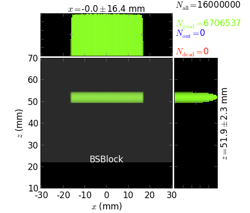
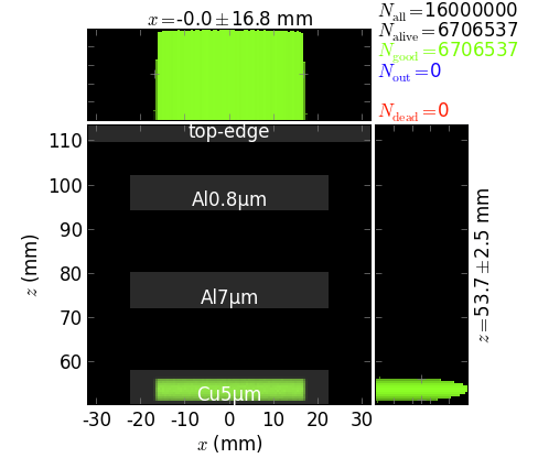
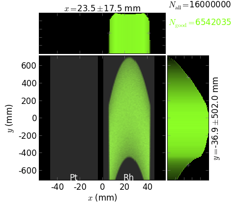
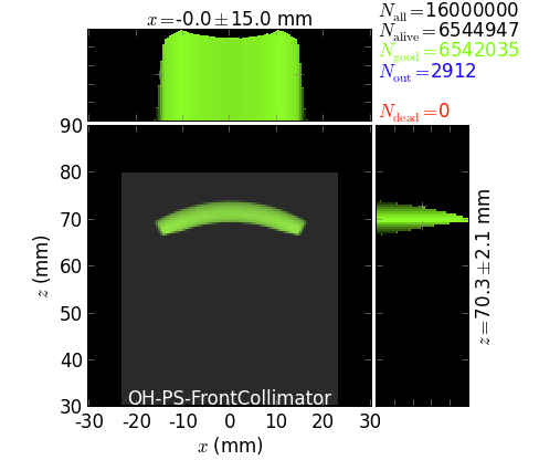
This script produces images at various positions along the beamline.

The following 13 images are:

1. FSM image after the front end with the projected absorbed rays (red) at

1. the fixed front end mask,

2. upstream half and

3. downstream half of the movable front end mask

2. footprint on VCM,

3. footprint on the 1st crystal of DCM,

4. footprint on the 2nd crystal of DCM,

5. beam at the Bremsstrahlung block,

6. image at the foil holder of 4-diode XBPM,

7. footprint on VFM,

8. front collimator of the photon shutter,

9. image at the reducer flange 100CF-to-40CF,

10. image at the EH 4-blade slit,

11. image at the focal (sample) point.

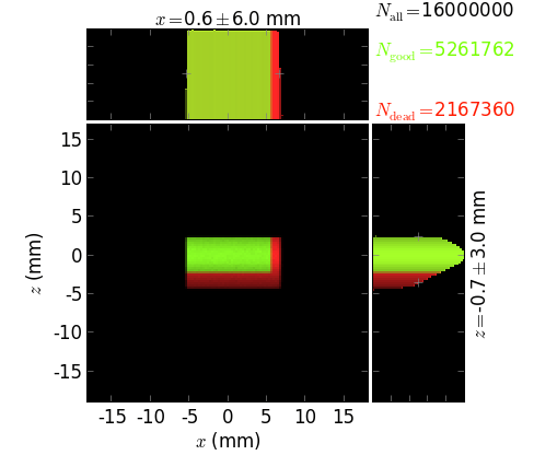
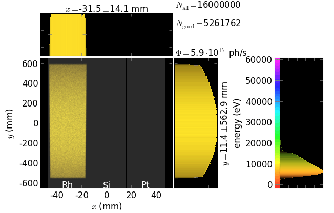
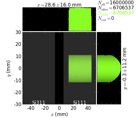
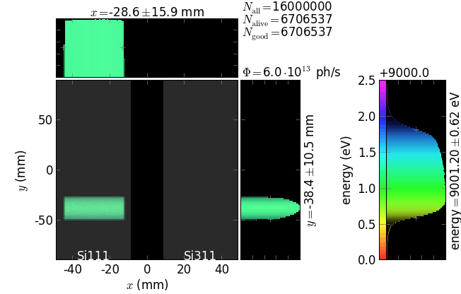
The script also exemplifies the usage of touch_beam() for finding the optimal size of slits.

Gratings, FZPs, Bragg-Fresnel optics, cPGM beamline

Files in \examples\withRaycing\09_Gratings

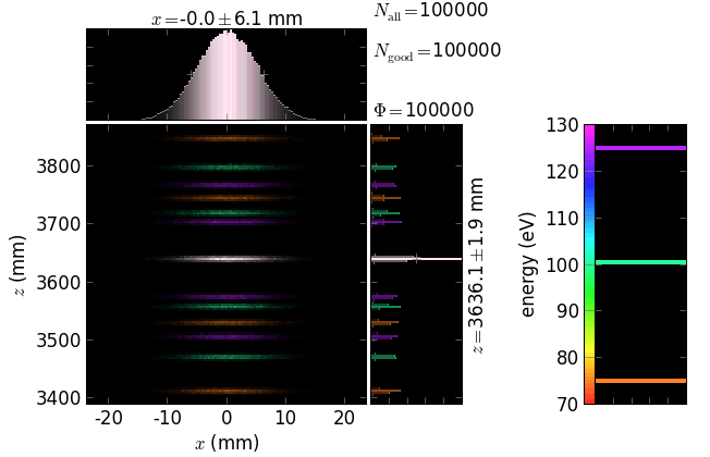
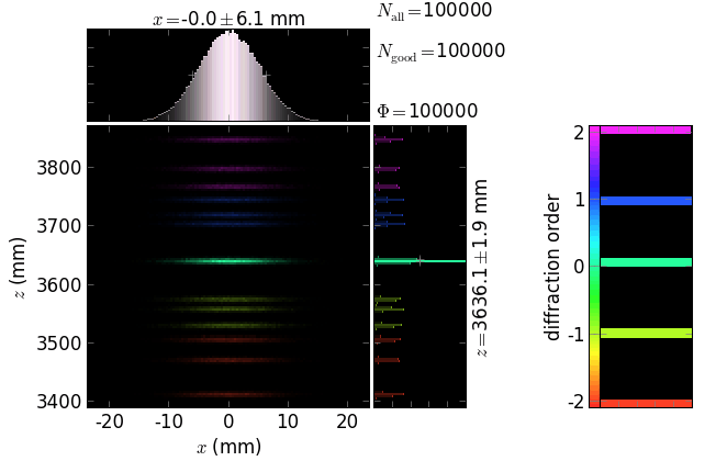
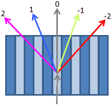
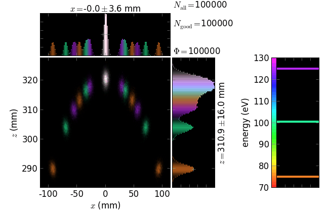
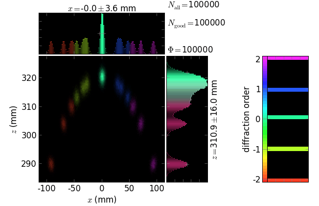
Simple gratings

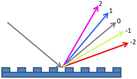
The following pictures exemplify simple gratings with the dispersion vector a) in the meridional plane and b) orthogonal to the meridional plane. Coloring is done by energy and by diffraction order.

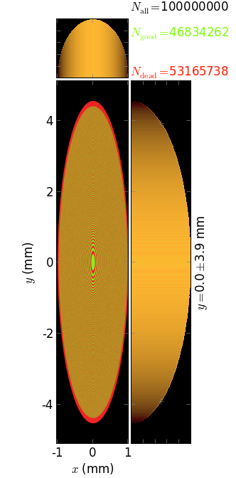
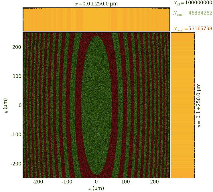
Fresnel Zone Plate

This example shows focusing of a quasi-monochromatic collimated beam by a normal (orthogonal to the beam) FZP. The energy distribution is uniform within 400 ± 5 eV. The focal length is 2 mm. The phase shift in the zones is variable and is relative to the central ray. As expected, the phase shift does not influence the focusing properties and can be selected at will.

zoomed footprint on FZP	focal spot

Bragg-Fresnel optics

One can combine an arbitrarily curved crystal surface, also (variably) asymmetrically cut, with a grating or zone structure on top of it. The following example shows a Fresnel zone structure that focuses a collimated beam at q = 20 m, whereas the Bragg crystal provides good energy resolution. One can easily study how the band width affects the focusing properties (not shown here).

Generic cPGM beamline

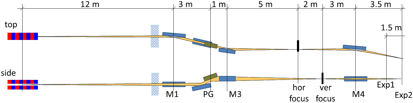
This example shows a generic cPGM beamline aligned for a fixed focus regime. The angles at the mirrors equal 2 degrees, c_ff = 2.25, the line density is 1221 mm^-1.

An energy scan at a given vertical slit (here, 30 µm) between M3 and M4. Shown are images at the slit and at the final focus ‘Exp2’:

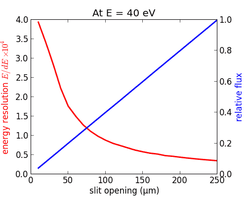
A vertical slit scan at a given energy (here, 40 eV) with a final dependency of energy resolution and flux on the slit size:

Multiple reflections

Files in \examples\withRaycing\10_MultipleReflect

Montel mirror

Montel mirror consists of two orthogonal mirrors positioned side-by-side. It is very similar to a KB mirror but more compact in the longitudinal direction. In a Montel mirror a part of the incoming beam is first reflected by one side of the mirror and then by the other side. Another part of the beam has the opposite reflection sequence. There are also single reflections on either side of the mirror. The non-sequential way of reflections makes such ray tracing impossible in most of ray-tracing programs.

The images below show the result of reflection by a Montel mirror consisting of a pair of parabolic mirrors. The mirrors can be selected by the user to have another shape. The coloring is by categories and the number of reflections. Notice a gap between the mirrors (here 0.2 mm) that transforms into a diagonal gap in the final image.

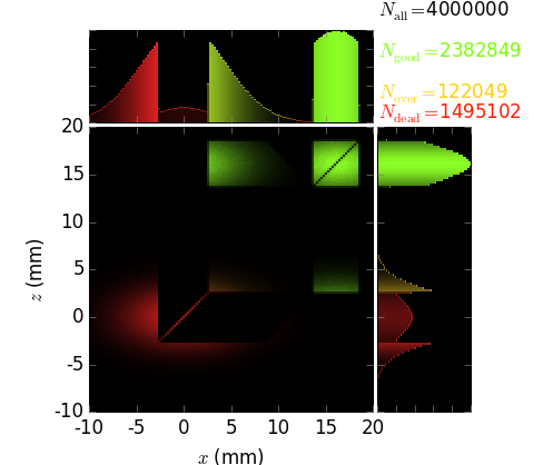
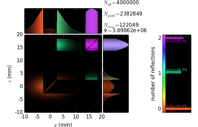
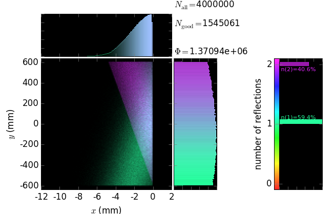
In the present example one can visualize the local footprints on either of the mirrors. The footprints are colored by the number of reflections.

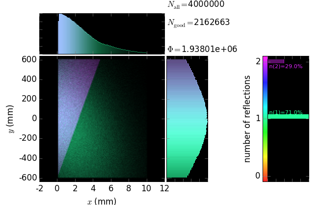
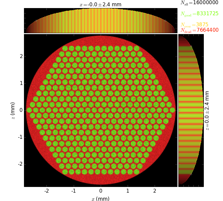
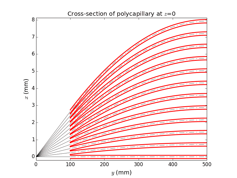
Polycapillary

This example also demonstrates the technique of propagating the beam through an array of non-sequential optical elements. These are 397 glass capillaries, close packed into a hexagonal bunch. The capillaries here serve for collimating a divergent beam (fluorescence) born at the origin. Each capillary here is parabolically (user-supplied shape) bent such that the left end tangents are directed towards the source and the right ends are parallel to the y axis. The capillary radius here is constant but can also be given by a user-function. The images below show the geometry of the polycapillary: the screen at the entrance that is colored by the categories of the exit beam (the green rays are reflected by the capillaries, the orange ones are transmitted without any reflection and the red ones are absorbed) and a longitudinal cross-section (note very different scales of x and y axes).

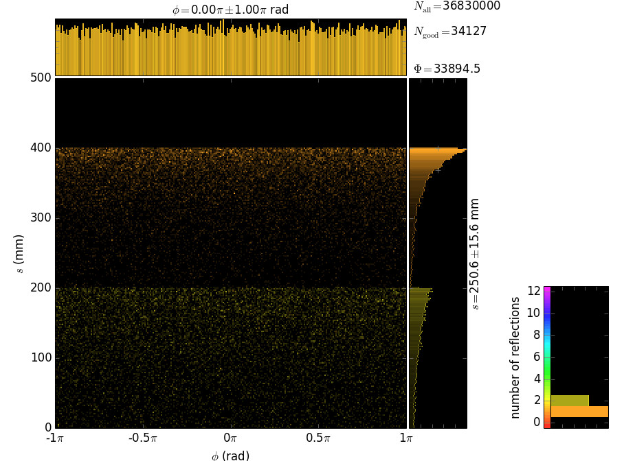
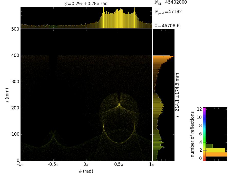
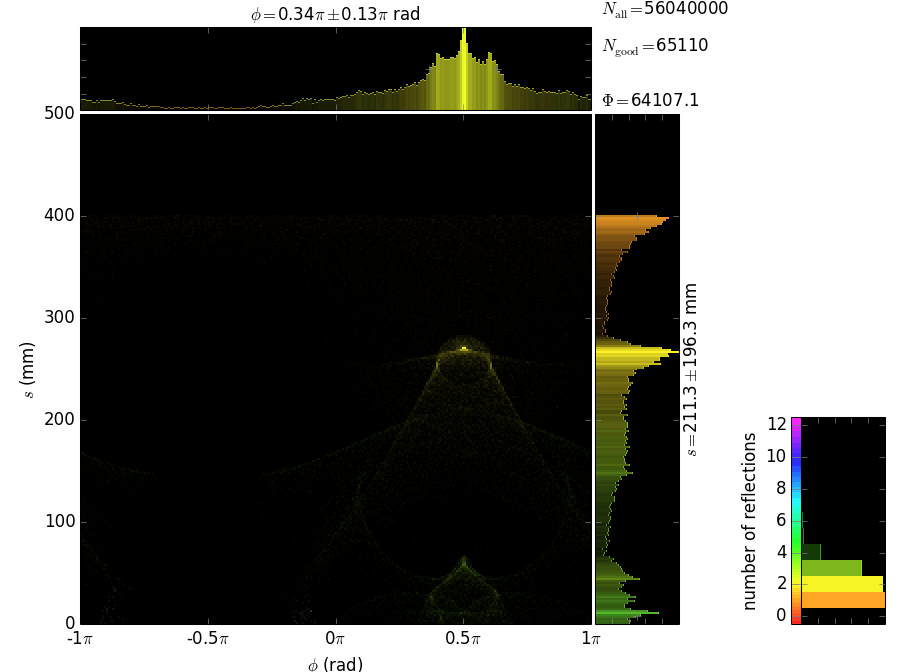
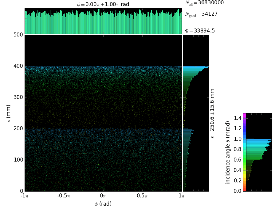
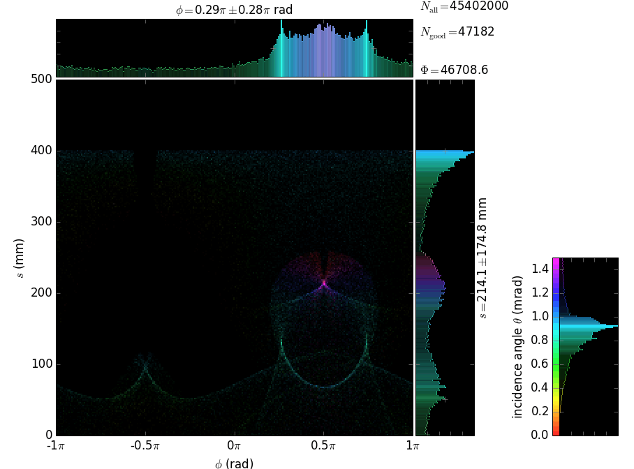
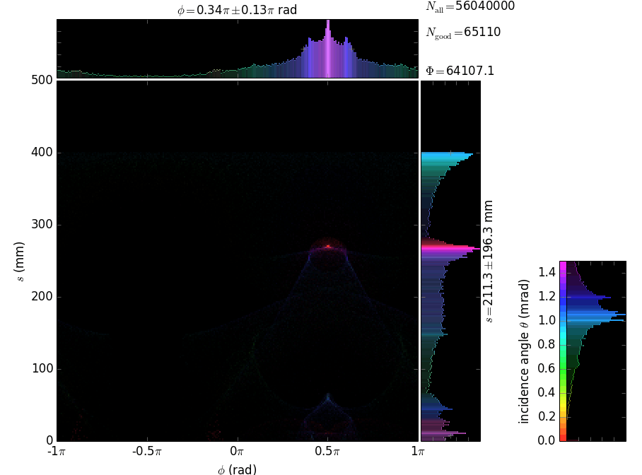
Each capillary reflects the rays many times until they are out. The local footprints over the capillary surface are vs. the polar angle and the longitudinal coordinate. The coloring is histogrammed over incidence angle and number of reflections. The longitudinal coordinate s has its zero at the exit from the capillary.

	layer 1	layer 6	layer 12
n refl
θ

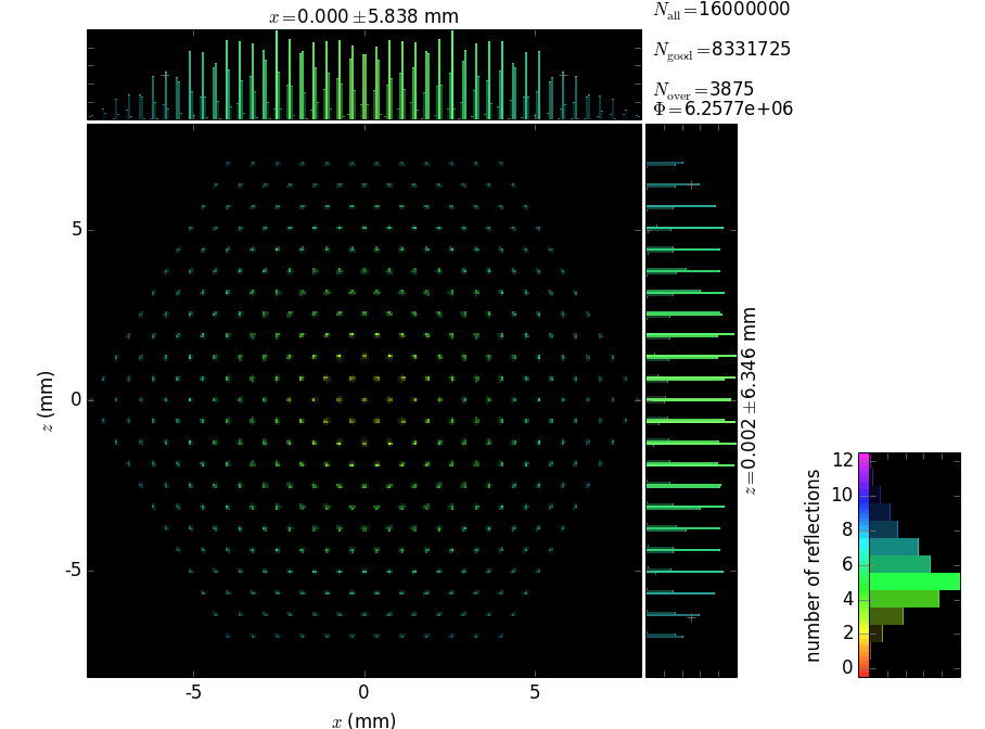
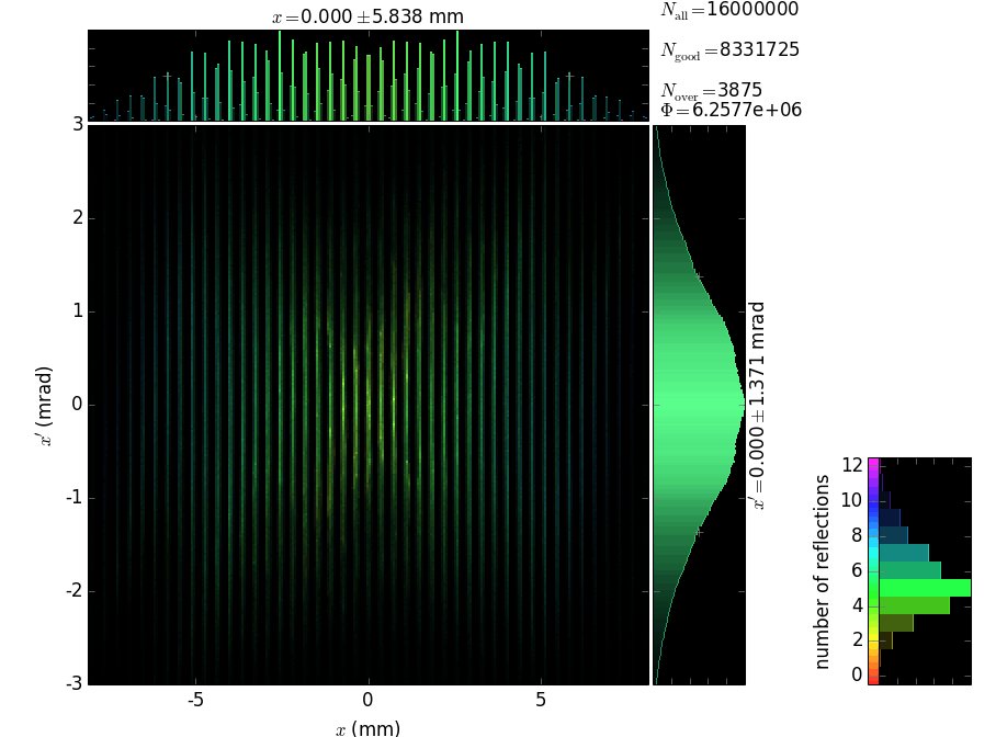
At the exit from the polycapillary the beam is expanded and attenuated at the periphery. The attenuation is due to the losses at each reflection; the number of reflections increases at the periphery, as shown by the colored histogram below. The phase space of the exit beam (shown is the horizontal one) shows the quality of collimation, see below. The divergence of ~1 mrad is large and cannot be efficiently used with a flat crystal analyzer.

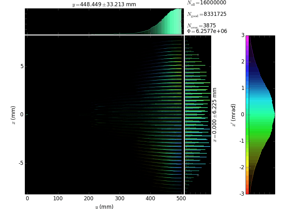
One may attempt to add a second-stage to collimate the beam with ~1 mrad divergence. However, this would not work because the rays collimated by a polycapillary have a very large distribution of the ray origins over the longitudinal direction y, as shown below.

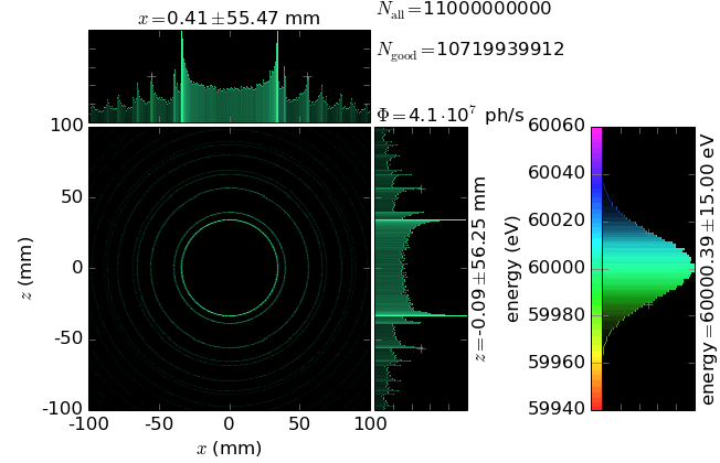
Powder Diffraction

Simulation of the real powder diffraction experiment on PETRA-III High Resolution Powder Diffraction Beamline P02.1. Uses Undulator source and double Laue Plate monochromator. Cerium Dioxide powder as the sample.

Warning

Heavy computational load. Requires OpenCL.