Raycing backend

Package raycing provides the internal backend of xrt. It defines beam sources in the module sources, rectangular and round apertures in apertures, optical elements in oes, material properties (essentially reflectivity, transmittivity and absorption coefficient) for interfaces and crystals in materials and screens in screens.

Coordinate systems

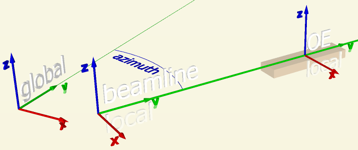
The following coordinate systems are considered (always right-handed):

1. The global coordinate system. It is arbitrary (user-defined) with one requirement driven by code simplification: Z-axis is vertical. For example, the system origin of Alba synchrotron is in the center of the ring at the ground level with Y-axis northward, Z upright and the units in mm.

   Note

   The positions of all optical elements, sources, screens etc. are given in the global coordinate system. This feature simplifies the beamline alignment when 3D CAD models are available.

2. The local systems.

   1. of the beamline. The local Y direction (the direction of the source) is determined by azimuth parameter of BeamLine – the angle measured cw from the global Y axis. The local beamline Z is also vertical and upward. The local beamline X is to the right. At azimuth = 0 the global system and the local beamline system are parallel to each other. In most of the supplied examples the global system and the local beamline system coincide.

   2. of an optical element. The origin is on the optical surface. Z is out-of-surface. At pitch, roll and yaw all zeros the local oe system and the local beamline system are parallel to each other.

      Note

      Pitch, roll and yaw rotations (correspondingly: Rx, Ry and Rz) are defined relative to the local axes of the optical element. The local axes rotate together with the optical element!

      Note

      The rotations are done in the following default sequence: yaw, roll, pitch. It can be changed by the user for any particular optical element. Sometimes it is necessary to define misalignment angles in addition to the positional angles. Because rotations do not commute, an extra set of angles may become unavoidable, which are applied after the positional rotations. See OE.

      The user-supplied functions for the surface height (z) and the normal as functions of (x, y) are defined in the local oe system.

   3. of other beamline elements: sources, apertures, screens. Z is upward and Y is along the beam line. The origin is given by the user. Usually it is on the original beam line.

xrt sequentially transforms beams (instances of Beam) – containers of arrays which hold beam properties for each ray. Geometrical beam properties such as x, y, z (ray origins) and a, b, c (directional cosines) as well as polarization characteristics depend on the above coordinate systems. Therefore, beams are usually represented by two different objects: one in the global and one in a local system.

Units

For the internal calculations, lengths are assumed to be in mm, although for reflection geometries and simple Bragg cases (thick crystals) this convention is not used. Angles are unitless (radians). Energy is in eV.

For plotting, the user may select units and conversion factors. The latter are usually automatically deduced from the units.

Beam categories

xrt discriminates rays by several categories:

1. good: reflected within the working optical surface;

2. out: reflected outside of the working optical surface, i.e. outside of a metal stripe on a mirror;

3. over: propagated over the surface without intersection;

4. dead: arrived below the optical surface and thus absorbed by the OE.

This distinction simplifies the adjustment of entrance and exit slits. The user supplies physical and optical limits, where the latter is used to define the out category (for rays between physical and optical limits). An alarm is triggered if the fraction of dead rays exceeds a specified level.

Scripting in python

The user of raycing must do the following:

1. Instantiate class BeamLine and fill it with sources, optical elements, screens etc.

2. Create a module-level function that returns a dictionary of beams – the instances of Beam. Assign this function to the module variable xrt.backends.raycing.run.run_process. The beams should be obtained by the methods shine() of a source, expose() of a screen, reflect() or multiple_reflect() of an optical element, propagate() of an aperture.

3. Use the keys in this dictionary for creating the plots (instances of XYCPlot). Note that at the time of instantiation the plots are just empty placeholders for the future 2D and 1D histograms.

4. Run run_ray_tracing() function for the created plots.

Additionally, the user may define a generator that will run a loop of ray tracing for changing geometry (mimics a real scan) or for different material properties etc. The generator should modify the beamline elements and output file names of the plots before yield. After the yield the plots are ready and the generator may use their fields, e.g. intensity or dE or dy or others to prepare a scan plot. Typically, this sequence is within a loop; after the loop the user may prepare the final scan plot using matplotlib functionality. The generator is given to run_ray_tracing() as a parameter.

See the supplied examples.

class xrt.backends.raycing.BeamLine(azimuth=0.0, height=0.0, alignE='auto')

Container class for beamline components. It also defines the beam line direction and height.

__init__(azimuth=0.0, height=0.0, alignE='auto')

azimuth: float

Is counted in cw direction from the global Y axis. At azimuth = 0 the local Y coincides with the global Y.

height: float

Beamline height in the global system.

alignE: float or ‘auto’

Energy for automatic alignment in [eV]. If ‘auto’, alignment energy is defined as the middle of the Source energy range. Plays a role if the pitch or bragg parameters of the energy dispersive optical elements were set to ‘auto’.

xrt.backends.raycing.run.run_process(beamLine)

Sources

Sampling strategies

There are three main strategies for creating samples of optical sources, depending on study purpose, implemented in xrt.

1. Monte Carlo sampling by intensity, or ray generation. This is the default mode of all synchrotron sources in xrt and is the best sampling strategy for ray tracing or hybrid wave propagation (when the wave part starts at a downstream optical element). Technically it is done by the acceptance-rejection method. In this method, the optical field is calculated in a 3D space – energy and two transverse angles – for a set of uniformly random values of these three variables within the predefined ranges. The transverse angles also get normally distributed angular shifts within the emittance distribution, independently for each ray. The acceptance random variable is uniformly sampled in the range from zero to the intensity maximum for each field sample, and the sample is accepted if the acceptance variable is below the sample intensity, otherwise it is rejected. The sampling continues until the requested number of samples is reached. The resulted space density of the samples (rays) is proportional to the field intensity. Simultaneously, this sampling gives the value of total flux as the product of the acceptance ratio times the 3D sample volume times the intensity maximum.

2. Uniform Monte Carlo sampling, or wave generation. This mode is necessary for wave propagation when it starts right from the source. The 3D calculation space – energy and two transverse angles – is sampled uniformly. This way of sampling is still possible to use for ray tracing, and it is even faster at the source as no samples are rejected, but it is less efficient at the downstream part of the beamline as a significant part of the samples (or even a majority of them) is of low intensity. The main usage pattern of this sampling is, however, for single electron (or macro electrons) field propagation (enabled by the source option filamentBeam=True), when all wave samples are attributed to the same electron with a single displacement within emittance distribution and a single shift of gamma (relative electron energy) within energy spread distribution. The flux is a sum of all intensities times the 3D sample volume over the number of samples.

3. Grid sampling. This is frequently a quick method for studying synchrotron sources in reciprocal space and energy that must be used with care as it is full of pitfalls. Grid samples can be obtained by intensities_on_mesh() method of the synchrotron source. Three aspects must be considered when making a grid. (i) For a sharp field distribution, e.g. for an undulator at zero emittance and zero electron beam energy spread, the sharp field rings may interfere with the grid (form moiré patterns) and result in false fringes in spectral flux density. In such cases, the grid has to be very finely spaced. (ii) When the electron beam emittance is non-zero, the calculated field values have to be convolved with the electron beam divergence; this convolution is done inside intensities_on_mesh(). Due to the edge effects of the convolution, the grid borders of the thickness of the doubled electron beam divergence must be discarded from the field arrays returned by intensities_on_mesh() and therefore these grid margins have to be added beforehand. (iii) The number of energy spread samples must be set sufficient for the used energy spread value, see the end of the next paragraph.

Electron beam energy spread is treated differently in the above three sampling strategies. In ray sampling, every ray gets its gamma sample (relative electron energy) of the normal energy spread distribution. In wave sampling, energy spread is sampled once for all wave samples when in filamentBeam regime and individually per wave sample otherwise. In grid sampling, a new grid dimension is introduced internally that contains samples of gamma within energy spread distribution with subsequent averaging over that dimension. Notice that a wide energy spread distribution (that can be a case for linacs) may require more energy spread samples (the parameter eSpreadNSamples of intensities_on_mesh()) than the default number 36 that is usually good for energy spread sigma of 0.1%. Because of this new dimension, the grid may become too large to fit into RAM, which might force the user to invoke the method intensities_on_mesh() in a loop that scans over individual photon energies.

Electron beam real space size is also treated differently in the above three sampling strategies. In ray sampling, every ray gets its transverse origin shift in the source plane within emittance distribution. In wave sampling, the wave source position is sampled once for all wave samples when in filamentBeam regime and individually per wave sample otherwise. In grid sampling, real space electron beam size is totally ignored.

See the example Undulator radiation through rectangular aperture, where several calculation methods are compared.

Geometric sources

Module sources defines the container class Beam that holds beam properties as numpy arrays and defines the beam sources. The sources are geometric sources in continuous and mesh forms and synchrotron sources.

The intensity and polarization of each ray are determined via coherency matrix. This way is appropriate for incoherent addition of rays, in which the components of the coherency matrix of different rays are simply added.

class xrt.backends.raycing.sources.Beam(nrays=100000, copyFrom=None, forceState=False, withNumberOfReflections=False, withAmplitudes=False, xyzOnly=False, bl=None)

Container for the beam arrays. x, y, z give the starting points. a, b, c give normalized vectors of ray directions (the source must take care about the normalization). E is energy. Jss, Jpp and Jsp are the components of the coherency matrix. The latter one is complex. Es and Ep are s and p field amplitudes (not always used). path is the total path length from the source to the last impact point. theta is the incidence angle. order is the order of grating diffraction. If multiple reflections are considered: nRefl is the number of reflections, elevationD is the maximum elevation distance between the rays and the surface as the ray travels from one impact point to the next one, elevationX, elevationY, elevationZ are the coordinates of the highest elevation points. If an OE uses a parametric representation, s, phi, r arrays store the impact points in the parametric coordinates.

concatenate(beam)

Adds beam to self. Useful when more than one source is presented.

export_beam(fileName, fformat='npy')

Saves the beam to a binary file. File format can be Numpy ‘npy’, Matlab ‘mat’ or python ‘pickle’. Matlab format should not be used for future imports in xrt as it does not allow correct load.

class xrt.backends.raycing.sources.GeometricSource

Implements a geometric source - a source with the ray origin, divergence and energy sampled with the given distribution laws.

__init__(bl=None, name='', center=(0, 0, 0), nrays=100000, distx='normal', dx=0.32, disty=None, dy=0, distz='normal', dz=0.018, distxprime='normal', dxprime=0.001, distzprime='normal', dzprime=0.0001, distE='lines', energies=(9000.0,), energyWeights=None, polarization='horizontal', filamentBeam=False, uniformRayDensity=False, pitch=0, roll=0, yaw=0)

bl: instance of BeamLine

name: str

center: tuple of 3 floats

3D point in global system

nrays: int

distx, disty, distz, distxprime, distzprime:

Linear (distx, disty, distz) and angular (distxprime, distzprime) source distributions. Accepted values: ‘normal’, ‘flat’, ‘annulus’ or None. If is None, the corresponding arrays remain with the values got at the instantiation of Beam. ‘annulus’ sets a uniform distribution for (x and z) or for (xprime and zprime) pairs. You can assign ‘annulus’ to only one member in the pair.

dx, dy, dz, dxprime, dzprime: float

Linear (dx, dy, dz) and angular (dxprime, dzprime) source sizes. For normal distribution is sigma or (sigma, cut_limit), for flat is full width or tuple (min, max), for annulus is tuple (rMin, rMax), otherwise is ignored.

distE: ‘normal’, ‘flat’, ‘lines’, None

energies: all in eV. (centerE, sigmaE) for distE = ‘normal’,

(minE, maxE) for distE = ‘flat’, a sequence of E values for distE = ‘lines’

energyWeights: 1-D array-like

Can be used together with distE = ‘lines’ to specify the weight of each line. Must be of the shape of energies.

polarization:

‘h[orizontal]’, ‘v[ertical]’, ‘+45’, ‘-45’, ‘r[ight]’, ‘l[eft]’, None, custom. In the latter case the polarization is given by a tuple of 4 components of the coherency matrix: (Jss, Jpp, Re(Jsp), Im(Jsp)).

filamentBeam: bool

If True the source generates coherent monochromatic wavefronts. Required for the wave propagation calculations.

uniformRayDensity: bool

If True, the radiation is sampled uniformly but with varying amplitudes, otherwise with the density proportional to intensity and with constant amplitudes. Required as True for wave propagation calculations. False is usual for ray-tracing. This parameter only affects normal distributions, as for flat and annulus distributions the density is already uniform. If you set it True, the size parameter (dx or dz) must be given as (sigma, cut_limit).

pitch, roll, yaw: float

rotation angles around x, y and z axes. Useful for canted sources.

class xrt.backends.raycing.sources.MeshSource

Implements a point source representing a rectangular angular mesh of rays. Primarily, it is meant for internal usage for matching the maximum divergence to the optical sizes of optical elements.

__init__(bl=None, name='', center=(0, 0, 0), minxprime=-0.0001, maxxprime=0.0001, minzprime=-0.0001, maxzprime=0.0001, nx=11, nz=11, distE='lines', energies=(9000.0,), energyWeights=None, polarization='horizontal', withCentralRay=True, autoAppendToBL=False)

bl: instance of BeamLine

name: str

center: tuple of 3 floats

3D point in global system

minxprime, maxxprime, minzprime, maxzprime: float

limits for the ungular distributions

nx, nz: int

numbers of points in x and z dircetions

distE: ‘normal’, ‘flat’, ‘lines’, None

energies, all in eV: (centerE, sigmaE) for distE = ‘normal’,

(minE, maxE) for distE = ‘flat’, a sequence of E values for distE = ‘lines’

energyWeights: 1-D array-like

Can be used together with distE = ‘lines’ to specify the weight of each line. Must be of the shape of energies.

polarization: ‘h[orizontal]’, ‘v[ertical]’, ‘+45’, ‘-45’, ‘r[ight]’,

‘l[eft]’, None, custom. In the latter case the polarization is given by a tuple of 4 components of the coherency matrix: (Jss, Jpp, Re(Jsp), Im(Jsp)).

withCentralRay: bool

if True, the 1st ray in the beam is along the nominal beamline direction

autoAppendToBL: bool

if True, the source is added to the list of beamline sources. Otherwise the user must manually start it with shine().

class xrt.backends.raycing.sources.CollimatedMeshSource(bl=None, name='', center=(0, 0, 0), dx=1.0, dz=1.0, nx=11, nz=11, distE='lines', energies=(9000.0,), energyWeights=None, polarization='horizontal', withCentralRay=True, autoAppendToBL=False)

Implements a source representing a mesh of collimated rays. Is similar to MeshSource.

class xrt.backends.raycing.sources.GaussianBeam(bl=None, name='', center=(0, 0, 0), w0=0.1, distE='lines', energies=(9000.0,), energyWeights=None, polarization='horizontal', pitch=0, roll=0, yaw=0)

Implements a Gaussian beam https://en.wikipedia.org/wiki/Gaussian_beam. It must be used for an already available set of 3D points which are obtained by prepare_wave() of a slit, oe or screen. See a usage example in \tests\raycing\laguerre_hermite_gaussian_beam.py.

__init__(bl=None, name='', center=(0, 0, 0), w0=0.1, distE='lines', energies=(9000.0,), energyWeights=None, polarization='horizontal', pitch=0, roll=0, yaw=0)

bl: instance of BeamLine

name: str

center: tuple of 3 floats

3D point in global system

w0: float or 2-sequence

Gaussian beam waist size. If a 2-sequence, the sizes refer to the horizontal and the vertical axes.

distE: ‘normal’, ‘flat’, ‘lines’, None

energies: all in eV. (centerE, sigmaE) for distE = ‘normal’,

(minE, maxE) for distE = ‘flat’, a sequence of E values for distE = ‘lines’

energyWeights: 1-D array-like

Can be used together with distE = ‘lines’ to specify the weight of each line. Must be of the shape of energies.

polarization:

‘h[orizontal]’, ‘v[ertical]’, ‘+45’, ‘-45’, ‘r[ight]’, ‘l[eft]’, None, custom. In the latter case the polarization is given by a tuple of 4 components of the coherency matrix: (Jss, Jpp, Re(Jsp), Im(Jsp)).

pitch, roll, yaw: float

rotation angles around x, y and z axes. Useful for canted sources.

class xrt.backends.raycing.sources.LaguerreGaussianBeam(*args, **kwargs)

Implements Laguerre-Gaussian beam https://en.wikipedia.org/wiki/Gaussian_beam. It must be used for an already available set of 3D points which are obtained by prepare_wave() of a slit, oe or screen. See a usage example in \tests\raycing\laguerre_hermite_gaussian_beam.py.

__init__(*args, **kwargs)

vortex: None or tuple(l, p)

specifies Laguerre-Gaussian beam with l the azimuthal index and p >= 0 the radial index.

class xrt.backends.raycing.sources.HermiteGaussianBeam(*args, **kwargs)

Implements Hermite-Gaussian beam https://en.wikipedia.org/wiki/Gaussian_beam. It must be used for an already available set of 3D points which are obtained by prepare_wave() of a slit, oe or screen. See a usage example in \tests\raycing\laguerre_hermite_gaussian_beam.py.

__init__(*args, **kwargs)

TEM: None or tuple(m, n)

specifies Hermite-Gaussian beam of order (m, n) referring to the x and y directions.

xrt.backends.raycing.sources.make_energy(distE, energies, nrays, filamentBeam=False, energyWeights=None)

Creates energy distributions with the distribution law given by distE. energies either determine the limits or is a sequence of discrete energies. If distE is ‘lines’, energyWeights can define the relative weights of the lines.

xrt.backends.raycing.sources.make_polarization(polarization, bo, nrays=100000)

Initializes the coherency matrix. The following polarizations are supported:

1. horizontal (polarization is a string started with ‘h’):

   \[\begin{split}J = \left( \begin{array}{ccc}1 & 0 \\ 0 & 0\end{array} \right)\end{split}\]

2. vertical (polarization is a string started with ‘v’):

   \[\begin{split}J = \left( \begin{array}{ccc}0 & 0 \\ 0 & 1\end{array} \right)\end{split}\]

3. at +45º (polarization = ‘+45’):

   \[\begin{split}J = \frac{1}{2} \left( \begin{array}{ccc}1 & 1 \\ 1 & 1\end{array} \right)\end{split}\]

4. at -45º (polarization = ‘-45’):

   \[\begin{split}J = \frac{1}{2} \left( \begin{array}{ccc}1 & -1 \\ -1 & 1\end{array} \right)\end{split}\]

5. right (polarization is a string started with ‘r’):

\[\begin{split}J = \frac{1}{2} \left( \begin{array}{ccc}1 & i \\ -i & 1\end{array} \right)\end{split}\]

5. left (polarization is a string started with ‘l’):

   \[\begin{split}J = \frac{1}{2} \left( \begin{array}{ccc}1 & -i \\ i & 1\end{array} \right)\end{split}\]

7. unpolarized (polarization is None):

   \[\begin{split}J = \frac{1}{2} \left( \begin{array}{ccc}1 & 0 \\ 0 & 1\end{array} \right)\end{split}\]

8. user-defined (polarization is 4-sequence with):

   \[\begin{split}J = \left( \begin{array}{ccc} {\rm polarization[0]} & {\rm polarization[2]} + i * {\rm polarization[3]} \\ {\rm polarization[2]} - i * {\rm polarization[3]} & {\rm polarization[1]}\end{array} \right)\end{split}\]

xrt.backends.raycing.sources.rotate_coherency_matrix(beam, indarr, roll)

Rotates the coherency matrix \(J\):

\[\begin{split}J = \left( \begin{array}{ccc} J_{ss} & J_{sp} \\ J^*_{sp} & J_{pp}\end{array} \right)\end{split}\]

by angle \(\phi\) around the beam direction as \(J' = R_{\phi} J R^{-1}_{\phi}\) with the rotation matrix \(R_{\phi}\) defined as:

\[\begin{split}R_{\phi} = \left( \begin{array}{ccc} \cos{\phi} & \sin{\phi} \\ -\sin{\phi} & \cos{\phi}\end{array} \right)\end{split}\]

xrt.backends.raycing.sources.copy_beam(beamTo, beamFrom, indarr, includeState=False, includeJspEsp=True)

Copies arrays of beamFrom to arrays of beamTo. The slicing of the arrays is given by indarr.

xrt.backends.raycing.sources.shrink_source(beamLine, beams, minxprime, maxxprime, minzprime, maxzprime, nx, nz)

Utility function that does ray tracing with a mesh source and shrinks its divergence until the footprint beams match to the optical surface. Parameters:

beamline: instance of BeamLine

beams: tuple of str

Dictionary keys in the result of run_process() corresponding to the wanted footprints.

minxprime, maxxprime, minzprime, maxzprime: float

Determines the size of the mesh source. This size can only be shrunk, not expanded. Therefore, you should provide it sufficiently big for your needs. Typically, min values are negative and max values are positive.

nx, nz: int

Sizes of the 2D mesh grid in x and z direction.

Returns an instance of MeshSource which can be used then for getting the divergence values.

Synchrotron sources

Note

In this section we consider z-axis to be directed along the beamline in order to be compatible with the cited works. Elsewhere in xrt z-axis looks upwards.

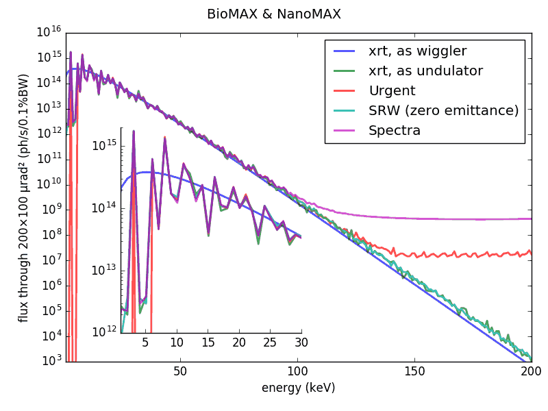
The synchrotron sources have two implementations: based on own fully pythonic or OpenCL aided calculations and based on external codes [Urgent] and [WS]. The latter codes have some drawbacks, as demonstrated in the section Comparison of synchrotron source codes, but nonetheless can be used for comparison purposes. If you are going to use them, the codes are freely available as parts of [XOP] package.

[Urgent] (1,2,3,4)

R. P. Walker, B. Diviacco, URGENT, A computer program for calculating undulator radiation spectral, angular, polarization and power density properties, ST-M-91-12B, July 1991, Presented at 4th Int. Conf. on Synchrotron Radiation Instrumentation, Chester, England, Jul 15-19, 1991

[WS]

R. J. Dejus, Computer simulations of the wiggler spectrum, Nucl. Instrum. Methods Phys. Res., Sect. A, 347 (1994) 56-60

[XOP] (1,2,3,4,5,6)

M. Sanchez del Rio, R. J. Dejus, XOP: A Multiplatform Graphical User Interface for Synchrotron Radiation Spectral and Optics Calculations, SPIE Proc. 3152 (1997) 148; web page: http://www.esrf.eu/Instrumentation/software/data-analysis/xop2.3.

The internal synchrotron sources are based on the following works: [Kim] and [Walker]. We use the general formulation for the flux distribution in 3-dimensional phase space (solid angle and energy) [Kim]:

\[\begin{split}\mathcal{F}(\theta,\psi,E) &= \alpha\frac{\Delta \omega}{\omega} \frac{I_e}{e^{-}}(A_{\sigma}^2 + A_{\pi}^2)\\\end{split}\]

For the bending magnets the amplitudes can be calculated analytically using the modified Bessel functions \(K_v(y)\):

\[\begin{split}\begin{bmatrix} A_{\sigma}\\ A_{\pi} \end{bmatrix} &= \frac{\sqrt{3}}{2\pi}\gamma\frac{\omega}{\omega_c} (1+\gamma^2\psi^2)\begin{bmatrix}-i K_{2/3}(\eta)\\ \frac{\gamma\psi}{\sqrt{1+\gamma^2\psi^2}} K_{1/3}(\eta)\end{bmatrix}\end{split}\]

where

\[\begin{split}\gamma &= \frac{E_e}{m_{e}c^2} = 1957E_e[{\rm GeV}]\\ \eta &= \frac{1}{2}\frac{\omega}{\omega_c}(1+\gamma^2\psi^2)^{3/2}\\ \omega_c &= \frac{3\gamma^{3}c}{2\rho}\\ \rho &= \frac{m_{e}c\gamma}{e^{-}B}\end{split}\]

with \(I_e\) - the current in the synchrotron ring, \(B\) - magnetic field strength, \(e^{-}, m_e\)- the electron charge and mass, \(c\) - the speed of light.

Wiggler radiation relies on the same equation considering each pole as a bending magnet with variable magnetic field/curvature radius: \(\rho(\theta) = \sin(\arccos(\theta\gamma/K))\), where \(K\) is deflection parameter. Total flux is multiplied then by \(2N\), where \(N\) is the number of wiggler periods.

For the undulator sources the amplitude integrals must be calculated numerically, starting from the magnetic field.

\[\begin{split}\begin{bmatrix} A_{\sigma}\\ A_{\pi} \end{bmatrix} &= \frac{1}{2\pi}\int\limits_{-\infty}^{+\infty}dt' \begin{bmatrix}\frac{[\textbf{n}\times[(\textbf{n}- \boldsymbol{\beta})\times\dot{\boldsymbol{\beta}}]]} {(1 - \textbf{n}\cdot\boldsymbol{\beta})^2}\end{bmatrix}_{x, y} e^{i\omega (t' + R(t')/c)}\end{split}\]

\[\begin{split}B_x &= B_{x0}\sin(2\pi z /\lambda_u + \phi),\\ B_y &= B_{y0}\sin(2\pi z /\lambda_u)\end{split}\]

the corresponding velosity components are

\[\begin{split}\beta_x &= \frac{K_y}{\gamma}\cos(\omega_u t),\\ \beta_y &= -\frac{K_x}{\gamma}\cos(\omega_u t + \phi)\\ \beta_z &= \sqrt{1-\frac{1}{\gamma^2}-\beta_{x}^{2}-\beta_{y}^{2}},\end{split}\]

where \(\omega_u = 2\pi c /\lambda_u\) - undulator frequency, \(\phi\) - phase shift between the magnetic field components. In this simple case one can consider only one period in the integral phase term replacing the exponential series by a factor \(\frac{\sin(N\pi\omega/\omega_1)}{\sin(\pi\omega/\omega_1)}\), where \(\omega_1 = \frac{2\gamma^2}{1+K_x^2/2+K_y^2/2+\gamma^2(\theta^2+\psi^2)} \omega_u\).

In the case of tapered undulator, the vertical magnetic field is multiplied by an additional factor \(1 - \alpha z\), that in turn results in modification of horizontal velocity and coordinate.

In the far-field approximation we consider the undulator as a point source and replace the distance \(R\) by a projection \(-\mathbf{n}\cdot\mathbf{r}\), where \(\mathbf{n} = [\theta,\psi,1-\frac{1}{2}(\theta^2+\psi^2)]\) - direction to the observation point, \(\mathbf{r} = [\frac{K_y}{\gamma}\sin(\omega_u t'), -\frac{K_x}{\gamma}\sin(\omega_u t' + \phi)\), \(\beta_m\omega t'-\frac{1}{8\gamma^2} (K_y^2\sin(2\omega_u t')+K_x^2\sin(2\omega_u t'+2\phi))]\) - electron trajectory, \(\beta_m = 1-\frac{1}{2\gamma^2}-\frac{K_x^2}{4\gamma^2}- \frac{K_y^2}{4\gamma^2}\).

Configurations with non-equivalent undulator periods i.e. tapered undulator require integration over full undulator length, similar approach is used for the near field calculations, where the undulator extension is taken into account and the phase component in the integral is taken in its initial form \(i\omega (t' + R(t')/c)\).

For the custom field configuratiuons, where the magnetic field components are tabulated as functions of longitudinal coordinate \(\textbf{B}=[B_{x}(z), B_{y}(z), B_{z}(z))]\), preliminary numerical calculation of the velocity and coordinate is nesessary. For that we solve the system of differential equations in the trajectory coordinate \(s\):

\[\begin{split}\frac{d^2}{ds^2} \begin{bmatrix}x\\ y\\ z\end{bmatrix} &= \frac{e^{-}}{\gamma m_{e} c} \begin{bmatrix}\beta_{y}B_{z}-B_{y}\\ -\beta_{x}B_{z}+B_{x}\\ -\beta_{y}B_{x}+\beta_{x}B_{y}\end{bmatrix}\end{split}\]

using the classical Runge-Kutta fourth-order method.

For the Undulator and custom field models we directly calculate the integral using the Clenshaw-Curtis quadrature, it proves to converge as quickly as the previously used Gauss-Legendre method, but the nodes and weights are calculated significantly faster. The size of the integration grid is evaluated at the points of slowest convergence (highest energy, maximum angular deviation i.e. a corner of the plot) before the start of intensity map calculation and then applied to all points. This approach creates certain computational overhead for the on-axis/low energy parts of the distribution but enables efficient parallelization and gives significant overall gain in performance. Initial evaluation typically takes just a few seconds, but might get much longer for custom magnetic fields and near edge calculations. If such heavy task is repeated many times for the given angular and energy limits it might make sense to note the evaluated size of the grid during the first run or call the test_convergence() method once, and then use the fixed grid by defining the gNodes at the init. Note also that the grid size will be automatically re-evaluated if any of the limits/electron energy/undulator deflection parameter or period length are redefined dynamically in the script.

Typical convergence threshold is defined by machine precision multiplied by the size of the integration grid. Default integration parameters proved to work very well in most cases, but may fail if the angular and/or energy limits are unreasonably wide. If in doubt, check the convergence with test_convergence(). See also a convergence study that justifies our automatic grid evaluation.

For the purpose of ray tracing (and this is not necessary for wave propagation) the undulator source size is calculated following [TanakaKitamura]. Their formulation includes dependence on electron beam energy spread. The effective linear and angular source sizes are given by

\[\begin{split}\Sigma &= \left(\sigma_e^2 + \sigma_r^2\right)^{1/2} =\left(\varepsilon\beta + \frac{\lambda L}{2\pi^2} [Q(\sigma_\epsilon/4)]^{4/3}\right)^{1/2}\\ \Sigma' &= \left({\sigma'_e}^2 + {\sigma'_r}^2\right)^{1/2} =\left(\varepsilon/\beta + \frac{\lambda}{2L} [Q(\sigma_\epsilon)]^2\right)^{1/2},\end{split}\]

where \(\varepsilon\) and \(\beta\) are the electron beam emittance and betatron function, the scaling function \(Q\) is defined as

\[Q(x) = \left(\frac{2x^2}{\exp(-2x^2)+(2\pi)^{1/2}x\ {\rm erf} (2^{1/2}x)-1}\right)^{1/2}\]

(notice \(Q(0)=1\)) and \(\sigma_\epsilon\) is the normalized energy spread

\[\sigma_\epsilon = 2\pi nN\sigma_E\]

i.e. the energy spread \(\sigma_E\) divided by the undulator bandwidth \(1/nN\) of the n-th harmonic, with an extra factor \(2\pi\). See an application example here.

Note

If you want to compare the source size with that by [SPECTRA], note that their radiation source size \(\sigma_r\) is by a factor of 2 smaller in order to be compatible with the traditional formula by [Kim]. In this aspect SPECTRA contradicts to their own paper [TanakaKitamura], see the paragraph after Eq(23).

[Kim] (1,2,3)

K.-J. Kim, Characteristics of Synchrotron Radiation, AIP Conference Proceedings, 184 (AIP, 1989) 565.

[Walker]

R. Walker, Insertion devices: undulators and wigglers, CAS - CERN Accelerator School: Synchrotron Radiation and Free Electron Lasers, Grenoble, France, 22-27 Apr 1996: proceedings (CERN. Geneva, 1998) 129-190.

[TanakaKitamura] (1,2,3)

T. Tanaka and H. Kitamura, Universal function for the brilliance of undulator radiation considering the energy spread effect, J. Synchrotron Rad. 16 (2009) 380–6.

class xrt.backends.raycing.sources.UndulatorUrgent

Undulator source that uses the external code Urgent. It has some drawbacks, as demonstrated in the section Comparison of synchrotron source codes, but nonetheless can be used for comparison purposes. If you are going to use it, the code is freely available as part of XOP package.

__init__(bl=None, name='UrgentU', center=(0, 0, 0), nrays=100000, period=32.0, K=2.668, Kx=0.0, Ky=0.0, n=12, eE=6.0, eI=0.1, eSigmaX=134.2, eSigmaZ=6.325, eEpsilonX=1.0, eEpsilonZ=0.01, uniformRayDensity=False, eMin=1500, eMax=81500, eN=1000, eMinRays=None, eMaxRays=None, xPrimeMax=0.25, zPrimeMax=0.1, nx=25, nz=25, path=None, mode=4, icalc=1, useZip=True, order=3, processes='auto')

The 1st instantiation of this class runs the Urgent code and saves its output into a “.pickle” file. The temporary directory “tmp_urgent” can then be deleted. If any of the Urgent parameters has changed since the previous run, the Urgent code is forced to redo the calculations.

bl: instance of BeamLine

Container for beamline elements. Sourcess are added to its sources list.

name: str

User-specified name, can be used for diagnostics output.

center: tuple of 3 floats

3D point in global system

nrays: int

the number of rays sampled in one iteration

period: float

Magnet period (mm).

K or Ky: float

Magnet deflection parameter (Ky) in the vertical field.

Kx: float

Magnet deflection parameter in the horizontal field.

n: int

Number of magnet periods.

eE: float

Electron beam energy (GeV).

eI: float

Electron beam current (A).

eSigmaX, eSigmaZ: float

rms horizontal and vertical electron beam sizes (µm).

eEpsilonX, eEpsilonZ: float

Horizontal and vertical electron beam emittance (nm rad).

eMin, eMax: float

Minimum and maximum photon energy (eV) used by Urgent.

eN: int

Number of photon energy intervals used by Urgent.

eMinRays, eMaxRays: float

The range of energies for rays. If None, are set equal to eMin and eMax. These two parameters are useful for playing with the energy axis without having to force Urgent to redo the calculations each time.

xPrimeMax, zPrimeMax: float

Half of horizontal and vertical acceptance (mrad).

nx, nz: int

Number of intervals in the horizontal and vertical directions from zero to maximum.

path: str

Full path to Urgent executable. If None, it is set automatically from the module variable xopBinDir.

mode: 1, 2 or 4

the MODE parameter of Urgent. If =1, UndulatorUrgent scans energy and reads the xz distribution from Urgent. If =2 or 4, UndulatorUrgent scans x and z and reads energy spectrum (angular density for 2 or flux through a window for 4) from Urgent. The meshes for x, z, and E are restricted in Urgent: nx,nz<50 and nE<5000. You may overcome these restrictions if you scan the corresponding quantities outside of Urgent, i.e. inside of this class UndulatorUrgent. mode = 4 is by far most preferable.

icalc: int

The ICALC parameter of Urgent.

useZip: bool

Use gzip module to compress the output files of Urgent. If True, the temporary storage takes much less space but a slightly bit more time.

order: 1 or 3

the order of the spline interpolation. 3 is recommended.

processes: int or any other type as ‘auto’

the number of worker processes to use. If the type is not int then the number returned by multiprocessing.cpu_count()/2 is used.

class xrt.backends.raycing.sources.WigglerWS

Wiggler source that uses the external code ws. It has some drawbacks, as demonstrated in the section Comparison of synchrotron source codes, but nonetheless can be used for comparison purposes. If you are going to use it, the code is freely available as part of XOP package.

__init__(*args, **kwargs)

Uses WS code. All the parameters are the same as in UndulatorUrgent.

class xrt.backends.raycing.sources.BendingMagnetWS

Bending magnet source that uses the external code ws. It has some drawbacks, as demonstrated in the section Comparison of synchrotron source codes, but nonetheless can be used for comparison purposes. If you are going to use it, the code is freely available as parts of XOP package.

__init__(*args, **kwargs)

Uses WS code.

B0: float

Field in Tesla.

K, n, period and nx:

Are set internally.

The other parameters are the same as in UndulatorUrgent.

class xrt.backends.raycing.sources.SourceBase

Base class for the Synchrotron Sources. Not to be called explicitly.

__init__(bl=None, name='GenericSource', center=(0, 0, 0), nrays=100000, eE=6.0, eI=0.1, eEspread=0.0, eSigmaX=None, eSigmaZ=None, eEpsilonX=1.0, eEpsilonZ=0.01, betaX=9.0, betaZ=2.0, eMin=5000.0, eMax=15000.0, distE='eV', xPrimeMax=0.5, zPrimeMax=0.5, R0=None, uniformRayDensity=False, filamentBeam=False, pitch=0, yaw=0, eN=51, nx=25, nz=25)

bl: instance of BeamLine

Container for beamline elements. Sourcess are added to its sources list.

name: str

User-specified name, can be used for diagnostics output.

center: tuple of 3 floats

3D point in global system.

nrays: int

The number of rays sampled in one iteration.

eE: float

Electron beam energy (GeV).

eI: float

Electron beam current (A).

eEspread: float

Energy spread relative to the beam energy, rms.

eSigmaX, eSigmaZ: float

rms horizontal and vertical electron beam sizes (µm). Alternatively, betatron functions can be specified instead of the electron beam sizes.

eEpsilonX, eEpsilonZ: float

Horizontal and vertical electron beam emittance (nm rad).

betaX, betaZ:

Betatron function (m). Alternatively, beam size can be specified.

R0: float

Distance center-to-screen for the near field calculations (mm). If None, the far field approximation (i.e. “usual” calculations) is used.

eMin, eMax: float

Minimum and maximum photon energy (eV). Used as band width for flux calculation.

distE: ‘eV’ or ‘BW’

The resulted flux density is per 1 eV or 0.1% bandwidth. For ray tracing ‘eV’ is used.

xPrimeMax, zPrimeMax:

Horizontal and vertical acceptance (mrad).

Note

The Monte Carlo sampling of the rays having their density proportional to the beam intensity can be extremely inefficient for sharply peaked distributions, like the undulator angular density distribution. It is therefore very important to restrict the sampled angular acceptance down to very small angles. Use this source only with reasonably small xPrimeMax and zPrimeMax!

uniformRayDensity: bool

If True, the radiation is sampled uniformly but with varying amplitudes, otherwise with the density proportional to intensity and with constant amplitudes. Required as True for wave propagation calculations. False is usual for ray-tracing.

filamentBeam: bool

If True the source generates coherent monochromatic wavefronts. Required as True for the wave propagation calculations in partially coherent regime.

pitch, yaw: float

rotation angles around x and z axis. Useful for canted sources.

intensities_on_mesh(energy='auto', theta='auto', psi='auto', harmonic=None, eSpreadSigmas=3.5, eSpreadNSamples=36, mode='constant', resultKind='Stokes')

Returns Stokes parameters (as a 4-list of arrays, when resultKind == ‘Stokes’) or intensities and OAM (Orbital Angular Momentum) matrix elements (as [Is, Ip, OAMs, OAMp, Es, Ep], when resultKind == ‘vortex’)in the shape (energy, theta, psi, [harmonic]), with theta being the horizontal mesh angles and psi the vertical mesh angles. Each one of the input arrays is a 1D array of an individually selectable length. Energy spread is sampled by a normal distribution and the resulting field values are averaged over it. eSpreadSigmas is sigma value of the distribution; eSpreadNSamples sets the number of samples. The resulted transverse field is convolved with angular spread by means of scipy.ndimage.filters.gaussian_filter. mode is a synonymous parameter of that filter that controls its behaviour at the borders.

Note

This method provides incoherent averaging over angular and energy spread of electron beam. The photon beam phase is lost here!

Note

We do not provide any internal mesh optimization, as mesh functions are not our core objectives. In particular, the angular meshes must be wider than the electron beam divergences in order to convolve the field distribution with the electron distribution. A warning will be printed (new in version 1.3.4) if the requested meshes are too narrow.

multi_electron_stack(energy='auto', theta='auto', psi='auto', harmonic=None, withElectronDivergence=True)

Returns Es and Ep in the shape (energy, theta, psi, [harmonic]). Along the 0th axis (energy) are stored “macro-electrons” that emit at the photon energy given by energy (constant or variable) onto the angular mesh given by theta and psi. The transverse field from each macro-electron gets individual random angular offsets dtheta and dpsi within the emittance distribution if withElectronDivergence is True and an individual random shift to gamma within the energy spread. The parameter self.filamentBeam is irrelevant for this method.

real_photon_source_sizes(energy='auto', theta='auto', psi='auto', method='rms')

Returns energy dependent arrays: flux, (dx’)², (dz’)², dx², dz². Depending on distE being ‘eV’ or ‘BW’, the flux is either in ph/s or in ph/s/0.1%BW, being integrated over the specified theta and psi ranges. The squared angular and linear photon source sizes are variances, i.e. squared sigmas. The latter two (linear sizes) are in mm**2.

class xrt.backends.raycing.sources.IntegratedSource

Base class for the Sources with numerically integrated amplitudes: SourceFromField and Undulator. Not to be called explicitly.

__init__(*args, **kwargs)

gp: float

Defines the relative precision of the integration (last significant digit). Undulator model converges down to 1e-6 and below. Custom field calculation may require setting the precision of 1e-3.

gNodes: int

Number of integration nodes in each of the integration intervals. If not provided at init, will be defined automatically.

targetOpenCL: None, str, 2-tuple or tuple of 2-tuples

assigns the device(s) for OpenCL accelerated calculations. None, if pyopencl is not wanted. Ignored if pyopencl is not installed. Accepts the following values:

1. a tuple (iPlatform, iDevice) of indices in the lists cl.get_platforms() and platform.get_devices(), see the section Calculations on GPU.

2. a tuple of tuples ((iP1, iD1), …, (iPn, iDn)) to assign specific devices from one or multiple platforms.

3. int iPlatform - assigns all devices found at the given platform.

4. ‘GPU’ - lets the program scan the system and select all found GPUs.

5. ‘CPU’ - similar to ‘GPU’. If one CPU exists in multiple platforms the program tries to select the vendor-specific driver.

6. ‘other’ - similar to ‘GPU’, used for Intel PHI and other OpenCL- capable accelerator boards.

7. ‘all’ - lets the program scan the system and assign all found devices. Not recommended, since the performance will be limited by the slowest device.

8. ‘auto’ - lets the program scan the system and make an assignment according to the priority list: ‘GPU’, ‘other’, ‘CPU’ or None if no devices were found. Used by default.

9. ‘SERVER_ADRESS:PORT’ - calculations will be run on remote server. See tests/raycing/RemoteOpenCLCalculation.

Warning

A good graphics or dedicated accelerator card is highly recommended! Special cases as wigglers by the undulator code, near field, wide angles and tapering are hardly doable on CPU.

Note

Consider the warnings and tips on using xrt with GPUs.

precisionOpenCL: ‘float32’ or ‘float64’, only for GPU.

Single precision (float32) should be enough in most cases. The calculations with doube precision are much slower. Double precision may be unavailable on your system. Tapering and Near Field calculations require double precision.

shine(toGlobal=True, withAmplitudes=True, fixedEnergy=False, wave=None, accuBeam=None)

Returns the source beam. If toGlobal is True, the output is in the global system. If withAmplitudes is True, the resulted beam contains arrays Es and Ep with the s and p components of the electric field.

fixedEnergy is either None or a value in eV. If fixedEnergy is specified, the energy band is not 0.1%BW relative to fixedEnergy, as probably expected but is given by (eMax - eMin) of the constructor.

wave and accuBeam are used in wave diffraction. wave is a Beam object and determines the positions of the wave samples. It must be obtained by a previous prepare_wave run. accuBeam is only needed with several repeats of diffraction integrals when the parameters of the filament beam must be preserved for all the repeats.

test_convergence(nMax=500000, withPlots=True, overStep=100)

This function evaluates the length of the integration grid required for convergence.

nMax: int

Maximum number of nodes.

withPlots: bool

Enables visualization.

overStep: int

Defines the number of extra points to calculate when the convergence is found. If None, calculation will proceed till nMax.

class xrt.backends.raycing.sources.Undulator

Undulator source. The computation is volumnous and thus a decent GPU is highly recommended.

__init__(*args, **kwargs)

period, n:

Magnetic period (mm) length and number of periods.

K, Kx, Ky: float

Deflection parameter for the vertical field or for an elliptical undulator.

B0x, B0y: float

Maximum magnetic field. If both K and B provided at the init, K value will be used.

phaseDeg: float

Phase difference between horizontal and vertical magnetic arrays. Used in the elliptical case where it should be equal to 90 or -90.

taper: tuple(dgap(mm), gap(mm))

Linear variation in undulator gap. None if tapering is not used. Pyopencl is recommended for tapering.

targetE: a tuple (Energy, harmonic{, isElliptical})

Can be given for automatic calculation of the deflection parameter. If isElliptical is not given, it is assumed as False (as planar).

xPrimeMaxAutoReduce, zPrimeMaxAutoReduce: bool

Whether to reduce too large angular ranges down to the feasible values in order to improve efficiency. It is highly recommended to keep them True.

get_SIGMA(E, onlyOddHarmonics=True, with0eSpread=False)

Calculates total linear source size, also including the effect of electron beam energy spread. Uses Tanaka and Kitamura, J. Synchrotron Rad. 16 (2009) 380–6.

E can be a value or an array. Returns a 2-tuple with x and y sizes.

get_SIGMAP(E, onlyOddHarmonics=True, with0eSpread=False)

Calculates total angular source size, also including the effect of electron beam energy spread. Uses Tanaka and Kitamura, J. Synchrotron Rad. 16 (2009) 380–6.

E can be a value or an array. Returns a 2-tuple with x and y sizes.

power_vs_K(energy, theta, psi, harmonics, Ks)

Calculates power curve – total power in W for all harmomonics at given K values (Ks). The power is calculated through the aperture defined by theta and psi opening angles within the energy range.

The result of this numerical integration depends on the used angular and energy meshes; you should check convergence. Internally, electron beam energy spread is also sampled by adding another dimension to the intensity array and making it 5-dimensional. You therefore may want to set energy spread to zero, it doesn’t affect the resulting power anyway.

Returns a 1D array corresponding to Ks.

tuning_curves(energy, theta, psi, harmonics, Ks)

Calculates tuning curves – maximum flux of given harmomonics at given K values (Ks). The flux is calculated through the aperture defined by theta and psi opening angles (1D arrays).

Returns two 2D arrays: energy positions and flux values. The rows correspond to Ks, the colums correspond to harmomonics.

class xrt.backends.raycing.sources.SourceFromField

Dedicated class for the sources based on a custom field table.

__init__(*args, **kwargs)

customField: float or str or tuple(fileName, kwargs) or numpy array.

If float, adds a constant longitudinal field. If str or tuple, expects table of field samples given as an Excel file or as text file. If given as a tuple or list, the 2nd member is a key word dictionary for reading Excel by pandas.read_excel() or reading text file by numpy.loadtxt(), e.g. dict(skiprows=4) for skipping the file header. The file must contain the columns with longitudinal coordinate in mm, {B_hor,} B_ver {, B_long}, all in T. The field can be provided as a numpy array with the same structure as the table from file.

class xrt.backends.raycing.sources.Wiggler

Wiggler source. The computation is reasonably fast and thus a GPU is not required and is not implemented.

__init__(*args, **kwargs)

Parameters are the same as in BendingMagnet except B0 and rho which are not required and additionally:

K: float

Deflection parameter

period: float

period length in mm.

n: int

Number of periods.

class xrt.backends.raycing.sources.BendingMagnet

Bending magnet source. The computation is reasonably fast and thus a GPU is not required and is not implemented.

__init__(*args, **kwargs)

B0: float

Magnetic field (T). Alternatively, specify rho.

rho: float

Curvature radius (m). Alternatively, specify B0.

Comparison of synchrotron source codes

Using xrt synchrotron sources on a mesh

The main modus operandi of xrt synchrotron sources is to provide Monte Carlo rays or wave samples. For comparing our sources with other codes – all of them are fully deterministic, being defined on certain meshes – we also supply mesh methods such as intensities_on_mesh, power_vs_K and tuning_curves. Note that we do not provide any internal mesh optimization, as these mesh functions are not our core objectives. Instead, the user themself should care about the proper mesh limits and step sizes. In particular, the angular meshes must be wider than the electron beam divergences in order to convolve the field distribution with the electron distribution of non-zero emittance. The above mentioned mesh methods will print a warning (new in version 1.3.4) if the requested meshes are too narrow.

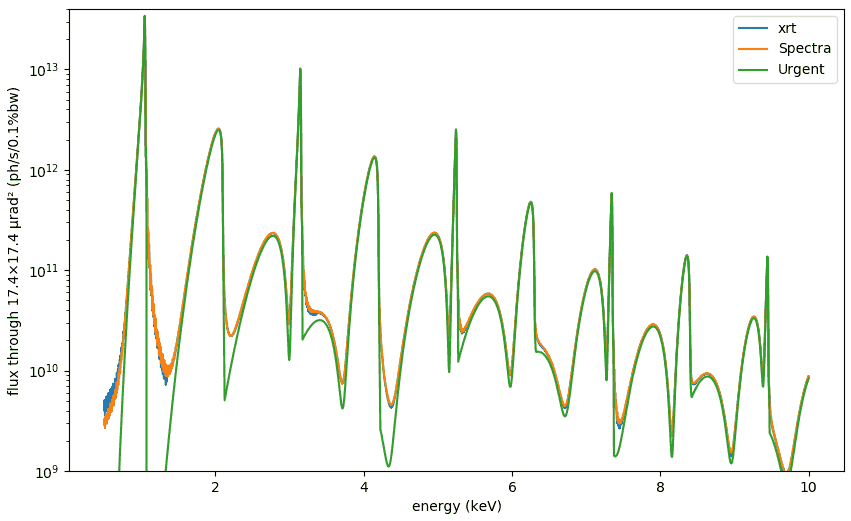
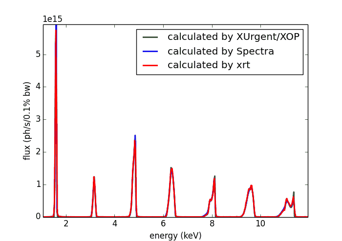
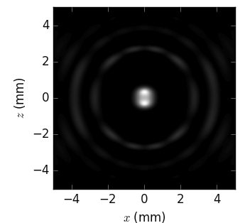
If you want to calculate flux through a narrow aperture, you first calculate intensities_on_mesh on wide enough angular meshes and then slice the intensity down to the needed aperture size. An example of such calculations is given in tests/raycing/test_undulator_on_mesh.py which produces the following plot (for a BESSY undulator, zero energy spread, as Urgent cannot take account of it):

Undulator spectrum across a harmonic

The above six classes result in ray distributions with the density of rays proportional to intensity. This requires an algorithm of Monte Carlo ray sampling that needs a 3D (two directions + energy) intensity distribution. The classes using the external mesh-based codes interpolate the source intensity pre-calculated over the user specified mesh. The latter three classes (internal implementation of synchrotron sources) do not require interpolation, which eliminates two problems: artefacts of interpolation and the need for the mesh optimization. However, this requires the calculations of intensity for each ray.

For bending magnet and wiggler sources these calculations are not heavy and are actually faster than 3D interpolation. See the absence of interpolation artefacts in Synchrotron sources in the gallery.

For an undulator the calculations are much more demanding and for a wide angular acceptance the Monte Carlo ray sampling can be extremely inefficient. To improve the efficiency, a reasonably small acceptance should be considered.

There are several codes that can calculate undulator spectra: [Urgent], [US], [SPECTRA]. There is a common problem about them that the energy spectrum may get strong distortions if calculated with a sparse spatial and energy mesh. SPECTRA code seems to provide the best reference for undulator spectra, which was used to optimize the meshes of the other codes. The final comparison of the resulted undulator spectra around a single harmonic is shown below.

[US] (1,2)

R. J. Dejus, US: Program to calculate undulator spectra. Part of XOP.

[SPECTRA] (1,2,3,4,5)

T. Tanaka and H. Kitamura, SPECTRA - a synchrotron radiation calculation code, J. Synchrotron Radiation 8 (2001) 1221-8.

Note

If you are going to use UndulatorUrgent, you should optimize the spatial and energy meshes! The resulted ray distribution is strongly dependent on them, especially on the energy mesh. Try different numbers of points and various energy ranges.

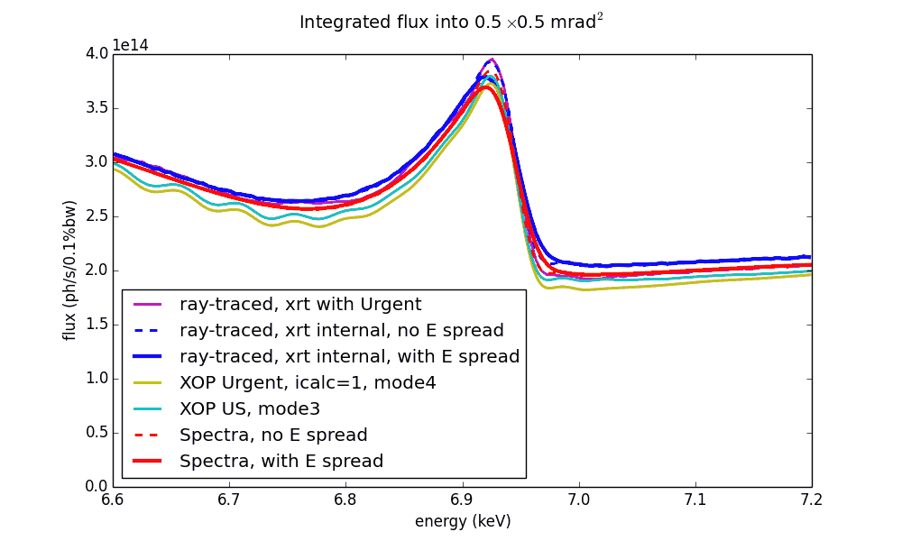
Undulator spectrum at very high energies

The codes [Urgent] and [SPECTRA] result in saturation at high energies (see the image below) thus leading to a divergent total power integral. The false radiation has a circular off-axis shape. To the contrary, xrt and [SRW] flux at high energies vanishes and follows the wiggler approximation. More discussion will follow in a future journal article about xrt.

Single-electron and multi-electron undulator radiation

Here we compare single-electron and multi-electron (i.e. with a finite electron beam size and energy spread) undulator radiation, as calculated by xrt and [SRW]. The calculations are done on a 3D mesh of energy (the long axis on the images below) and two transverse angles. Notice also the duration of execution given below each image. The 3D mesh was the following: theta = 321 point, -0.3 to +0.3 mrad, psi = 161 point, -0.15 to +0.15 mrad, energy: 301 point 1.5 to 4.5 keV.

[SRW] (1,2,3)

O. Chubar, P. Elleaume, Accurate And Efficient Computation Of Synchrotron Radiation In The Near Field Region, proc. of the EPAC98 Conference, 22-26 June 1998, p.1177-1179.

	SRW	xrt
single electron
	execution time 974 s	execution time 17.4 s
non-zero emittance
	execution time 65501 s (sic)	execution time 18.6 s
non-zero emittance, non-zero energy spread
	execution time 66180 s (sic)	execution time 216 s

Undulator spectrum with tapering

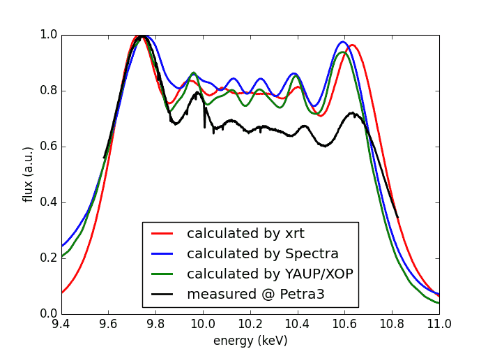
The spectrum can be broadened by tapering the magnetic gap. The figure below shows a comparison of xrt with [SPECTRA], [YAUP] and experimental measurements [exp_taper]. The gap values and the taper were slightly varied in all three codes to reach the best match with the experimental curve. We had to do so because in the other codes taper is not clearly defined (where is the gap invariant – at the center or at one of the ends?) and also because the nominal experimental gap and taper are not fully trustful.

[YAUP]

B. I. Boyanov, G. Bunker, J. M. Lee, and T. I. Morrison, Numerical Modeling of Tapered Undulators, Nucl. Instr. Meth. A339 (1994) 596-603.

[exp_taper]

Measured on 27 Nov 2013 on P06 beamline at Petra 3, R. Chernikov and O. Müller, unpublished.

The source code is in examples\withRaycing\01_SynchrotronSources

Notice that not only the band width is affected by tapering. Also the transverse distribution attains inhomogeneity which varies with energy, see the animation below. Notice also that such a picture is sensitive to emittance; the one below was calculated for the emittance of Petra III ring.

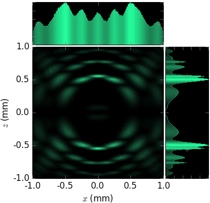
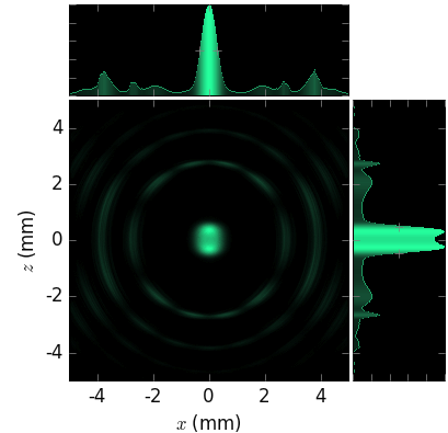
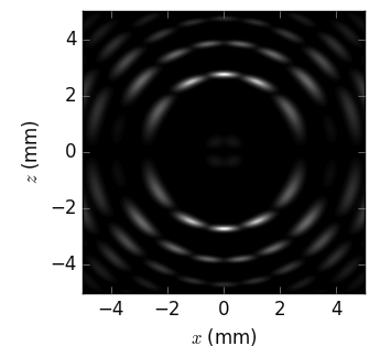
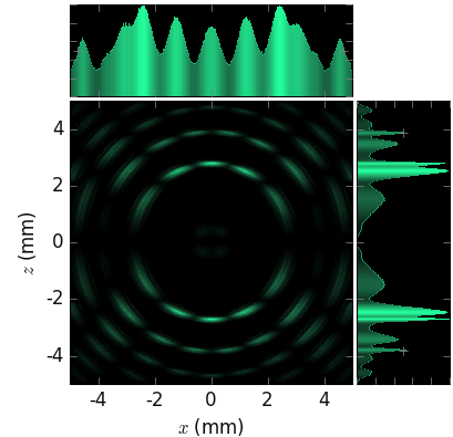
Undulator spectrum in transverse plane

The codes calculating undulator spectra – [Urgent], [US], [SPECTRA] – calculate either the spectrum of flux through a given aperture or the transversal distribution at a fixed energy. It is not possible to simultaneously have two dependencies: on energy and on transversal coordinates.

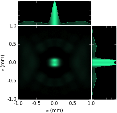
Whereas xrt gives equal results to other codes in such univariate distributions as flux through an aperture:

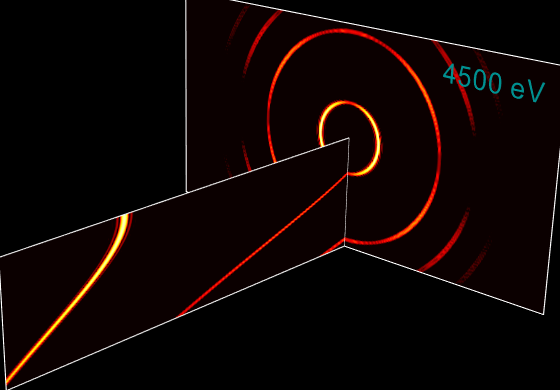
… and transversal distribution at a fixed energy:

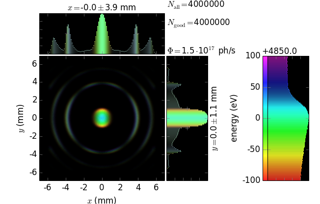
	SPECTRA	xrt
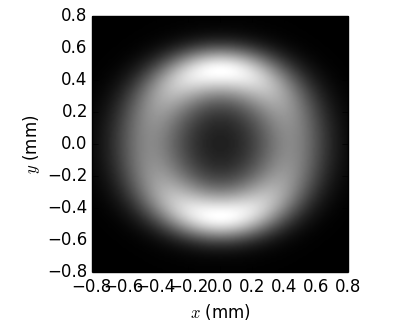
E = 4850 eV (3rd harmonic)
E = 11350 eV (7th harmonic)

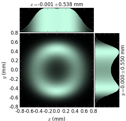
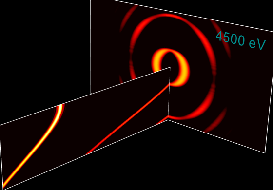
…, xrt can combine the two distributions in one image and thus be more informative:

	zoom in	zoom out
E ≈ 4850 eV (3rd harmonic)
E ≈ 11350 eV (7th harmonic)

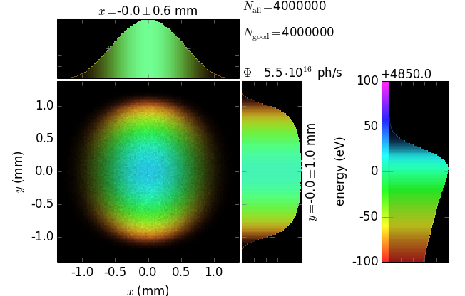
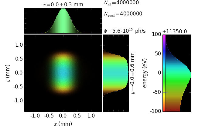
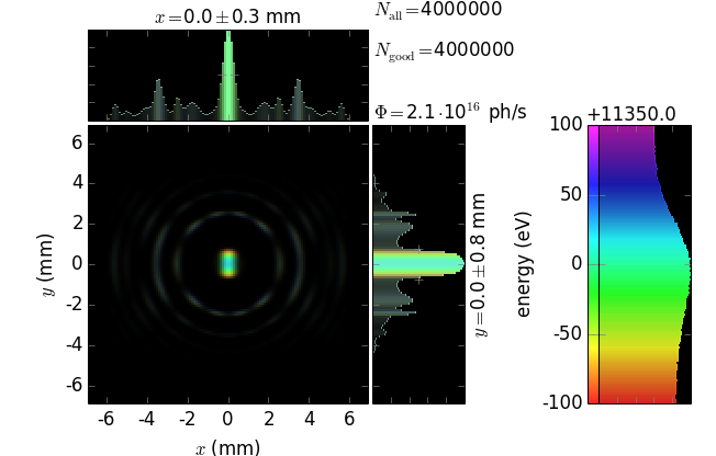
In particular, it is seen that divergence strongly depends on energy, even for such a narrow energy band within one harmonic. It is also seen that the maximum flux corresponds to slightly off-axis radiation (greenish color) but not to the on-axis radiation (bluish color).

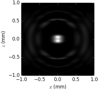
Undulator radiation in near field

Notice that on the following pictures the p-polarized flux is only ~6% of the total flux.

at 5 m	SPECTRA	xrt
far field at 5 m, full flux
far field at 5 m, p-polarized
near field at 5 m, full flux
near field at 5 m, p-polarized

at 25 m	SPECTRA	xrt
far field at 25 m, full flux
far field at 25 m, p-polarized
near field at 25 m full flux
near field at 25 m, p-polarized

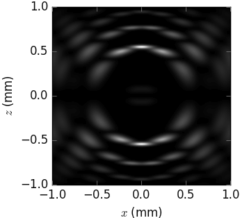
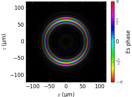
Field phase in near field

The phase of the radiation field on a flat screen as calculated by the three codes is compared below. Notice that the visualization (brightness=intensity, color=phase) is not by SRW and SPECTRA but was done by us.

SRW [SRW]	SPECTRA	xrt

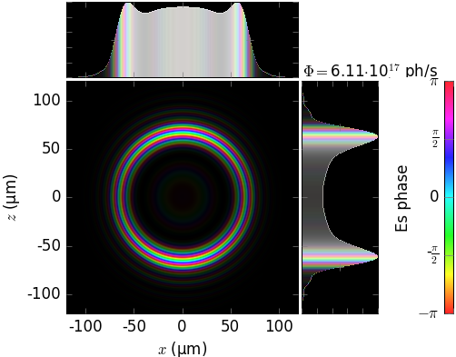
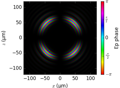
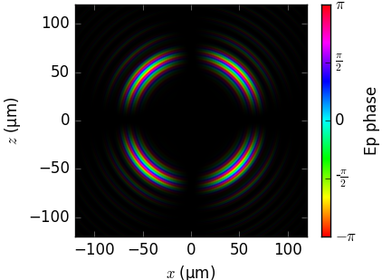
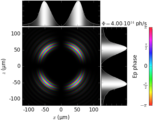
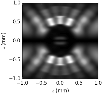
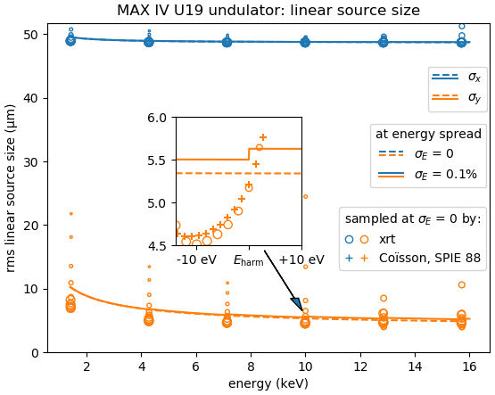
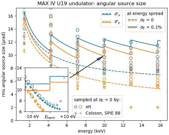
Undulator source size dependent on energy spread and detuning

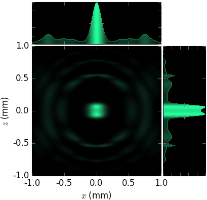
The linear and angular source sizes, as calculated with equations from [TanakaKitamura] (summarized here) for a U19 undulator in MAX IV 3 GeV ring (\(E_1\) = 1429 eV) with \(\varepsilon_x\) = 263 pmrad, \(\varepsilon_y\) = 8 pmrad, \(\beta_x\) = 9 m and \(\beta_y\) = 2 m, are shown below. Energy spread mainly affects the angular sizes and not the linear ones.

The calculated sizes were further compared with those of the sampled field (circles) at variable energies around the nominal harmonic positions, i.e. at so called undulator detuning. To get the photon source size distribution, the angular distributions of Es and Ep field amplitudes were Fourier transformed, as described in [Coïsson]. The sampled field sizes strongly vary due to undulator detuning, as is better seen on the magnified insets. The size variation by detuning is the underlying reason for the size dependence on energy spread: with a non-zero energy spread the undulator becomes effectively detuned for some electrons depending on their velocity.

The size of the circles is proportional to the total flux normalized to the maximum at each respective harmonic. It sharply decreases at the higher energy end of a harmonic and has a long tail at the lower energy end, in accordance with the above examples.

The effect of energy detuning from the nominal undulator harmonic energy on the photon source size is compared to the results by Coïsson [Coïsson] (crosses in the figures below). He calculated the sizes for a single electron field, and thus without emittance and energy spread. For comparison, we also sampled the undulator field at zero energy spread and emittance.

[Coïsson] (1,2)

R. Coïsson, Effective phase space widths of undulator radiation, Opt. Eng. 27 (1988) 250–2.

Optical elements

Module oes defines a generic optical element in class OE. Its methods serve mainly for propagating the beam downstream the beamline. This is done in the following sequence: for each ray transform the beam from global to local coordinate system, find the intersection point with the OE surface, define the corresponding state of the ray, calculate the new direction, rotate the coherency matrix to the local s-p basis, calculate reflectivity or transmittivity and apply it to the coherency matrix, rotate the coherency matrix back and transform the beam from local to the global coordinate system.

Module oes defines also several other optical elements with various geometries.

class xrt.backends.raycing.oes.OE

The main base class for an optical element. It implements a generic flat mirror, crystal, multilayer or grating.

__init__(bl=None, name='', center=[0, 0, 0], pitch=0, roll=0, yaw=0, positionRoll=0, rotationSequence='RzRyRx', extraPitch=0, extraRoll=0, extraYaw=0, extraRotationSequence='RzRyRx', alarmLevel=None, surface=None, material=None, alpha=None, limPhysX=[-1000.0, 1000.0], limOptX=None, limPhysY=[-1000.0, 1000.0], limOptY=None, isParametric=False, shape='rect', gratingDensity=None, order=None, shouldCheckCenter=False, targetOpenCL=None, precisionOpenCL='float64')

bl: instance of BeamLine

Container for beamline elements. Optical elements are added to its oes list.

name: str

User-specified name, occasionally used for diagnostics output.

center: 3-sequence of floats

3D point in global system. Any two coordinates can be ‘auto’ for automatic alignment.

pitch, roll, yaw: floats

Rotations Rx, Ry, Rz, correspondingly, defined in the local system. If the material belongs to Crystal, pitch can be calculated automatically if alignment energy is given as a single element list [energy]. If ‘auto’, the alignment energy will be taken from beamLine.alignE.

positionRoll: float

A global roll used for putting the OE upside down (=np.pi) or at horizontal deflection (=[-]np.pi/2). This parameter does the same rotation as roll. It is introduced for holding large angles, as π or π/2 whereas roll is meant for smaller [mis]alignment angles.

rotationSequence: str, any combination of ‘Rx’, ‘Ry’ and ‘Rz’

Gives the sequence of rotations of the OE around the local axes. The sequence is read from left to right (do not consider it as an operator). When rotations are more than one, the final position of the optical element depends on this parameter.

extraPitch, extraRoll, extraYaw, extraRotationSequence:

Similar to pitch, roll, yaw, rotationSequence but applied after them. This is sometimes necessary because rotations do not commute. The extra angles were introduced for easier misalignment after the initial positioning of the OE.

alarmLevel: float or None

Allowed fraction of incident rays to be absorbed by OE. If exceeded, an alarm output is printed in the console.

surface: None or sequence of str

If there are several optical surfaces, such as metalized stripes on a mirror, these are listed here as names; then also the optical limits must all be given by sequences of the same length if not None.

material: None or sequence of material objects

The material(s) must have get_amplitude() or get_refractive_index() method. If not None, must correspond to surface. If None, the reflectivities are equal to 1.

alpha: float

Asymmetry angle for a crystal OE (rad). Positive sign is for the atomic planes’ normal looking towards positive y.

limPhysX and limPhysY: [min, max] where min, max are

floats or sequences of floats Physical dimension = local coordinate of the corresponding edge. Can be given by sequences of the length of surface. You do not have to provide the limits, although they may help in finding intersection points, especially for (strongly) curved surfaces.

limOptX and limOptY: [min, max] where min, max are

floats or sequences of floats Optical dimension = local coordinate of the corresponding edge. Useful when the optical surface is smaller than the whole surface, e.g. for metalized stripes on a mirror.

isParametric: bool

If True, the OE is defined by parametric equations rather than by z(x, y) function. For example, parametric representation is useful for describing closed surfaces, such as capillaries. The user must supply the transformation functions param_to_xyz() and xyz_to_param() between local (x, y, z) and (s, phi, r) and the parametric surface local_r dependent on (s, phi). The exact meaning of these three new parameters is up to the user because this meaning is self-contained in the above mentioned user-supplied functions. For example, these can be viewed as cylindrical-like coordinates, where s is a running coordinate on a 3D axial curve, phi and r are polar coordinates in planes normal to the axial curve and crossing that curve at point s. Class SurfaceOfRevolution gives an example of the transformation functions and represents a useful kind of parametric surface. The methods local_n() (surface normal) and local_g() (grating vector, if used for this OE) return 3D vectors in local xyz space but now the two input coordinate parameters are s and phi. The limits [limPhysX, limOptX] and [limPhysY, limOptY] still define, correspondingly, the limits in local x and y. The local beams (footprints) will additionally contain s, phi and r arrays.

shape: str or list of [x, y] pairs

The shape of OE. Supported: ‘rect’, ‘round’ or a list of [x, y] pairs for an arbitrary shape.

gratingDensity: None or list

If material kind = ‘grating’, its density can be defined as list [axis, ρ₀, P₀, P₁, …], where ρ₀ is the constant line density in inverse mm, P₀ – P_n are polynom coefficients defining the line density variation, so that for a given axis

\[\rho_x = \rho_0\cdot(P_0 + 2 P_1 x + 3 P_2 x^2 + ...).\]

Example: [‘y’, 800, 1] for the grating with constant spacing along the ‘y’ direction; [‘y’, 1200, 1, 1e-6, 3.1e-7] for a VLS grating. The length of the list determines the polynomial order.

order: int or sequence of ints

The order(s) of grating, FZP or Bragg-Fresnel diffraction.

shouldCheckCenter: bool

This is a leagcy parameter designed to work together with alignment stages – classes in module stages – which modify the orientation of an optical element. if True, invokes checkCenter method for checking whether the oe center lies on the original beam line. checkCenter implies vertical deflection and ignores any difference in height. You should override this method for OEs of horizontal deflection.

targetOpenCL: None, str, 2-tuple or tuple of 2-tuples

pyopencl can accelerate the search for the intersections of rays with the OE. If pyopencl is used, targetOpenCL is a tuple (iPlatform, iDevice) of indices in the lists cl.get_platforms() and platform.get_devices(), see the section Calculations on GPU. None, if pyopencl is not wanted. Ignored if pyopencl is not installed.

precisionOpenCL: ‘float32’ or ‘float64’, only for GPU.

Single precision (float32) should be enough. So far, we do not see any example where double precision is required. The calculations with double precision are much slower. Double precision may be unavailable on your system.

local_g(x, y, rho=-100.0)

For a grating, gives the local reciprocal groove vector (without 2pi!) in 1/mm at (x, y) position. The vector must lie on the surface, i.e. be orthogonal to the normal. Typically is overridden in the derived classes or defined in Material class. Returns a 3-tuple of floats or of arrays of the length of x and y.

local_n(x, y)

Determines the normal vector of OE at (x, y) position. Typically is overridden in the derived classes. If OE is an asymmetric crystal, local_n must return 2 normals as a 6-sequence: the 1st one of the atomic planes and the 2nd one of the surface. Note the order!

If isParametric in the constructor is True, local_n() still returns 3D vector(s) in local xyz space but now the two input coordinate parameters are s and phi.

The result is a 3-tuple or a 6-tuple. Each element is either a scalar or an array of the length of x and y.

local_n_distorted(x, y)

Distortion to the local normal. If isParametric in the constructor is True, the input arrays are understood as (s, phi).

Distortion can be given in two ways and is signaled by the length of the returned tuple:

1. As d_pitch and d_roll rotation angles of the normal (i.e. rotations Rx and Ry). A tuple of the two arrays must be returned. This option is also suitable for parametric coordinates because the two rotations will be around Cartesian axes and the local normal (local_n) is also a 3D vector in local xyz space.

2. As a 3D vector that will be added to the local normal calculated at the same coordinates. The returned vector can have any length, not necessarily unity. As for local_n, the 3D vector is in local xyz space even for a parametric surface. The resulted vector local_n + local_n_distorted will be normalized internally before calculating the reflected beam direction. A tuple of 3 arrays must be returned.

local_z(x, y)

Determines the surface of OE at (x, y) position. Typically is overridden in the derived classes. Must return either a scalar or an array of the length of x and y.

multiple_reflect(beam=None, maxReflections=1000, needElevationMap=False, returnLocalAbsorbed=None)

Does the same as reflect() but with up to maxReflections reflection on the same surface.

The returned beam has additional fields: nRefl for the number of reflections, elevationD for the maximum elevation distance between the rays and the surface as the ray travels between the impact points, elevationX, elevationY, elevationZ for the coordinates of the maximum elevation points.

returnLocalAbsorbed: None or int

If not None, returns the absorbed intensity in local beam.

prepare_wave(prevOE, nrays, shape='auto', area='auto', rw=None)

Creates the beam arrays used in wave diffraction calculations. prevOE is the diffracting element: a descendant from OE, RectangularAperture or RoundAperture. nrays: if int, specifies the number of randomly distributed samples the surface within self.limPhysX limits; if 2-tuple of ints, specifies (nx, ny) sizes of a uniform mesh of samples.

reflect(beam=None, needLocal=True, noIntersectionSearch=False, returnLocalAbsorbed=None)

Returns the reflected or transmitted beam as \(\vec{out}\) in global and local (if needLocal is true) systems.

Mirror [wikiSnell]:

\[\begin{split}\vec{out}_{\rm reflect} &= \vec{in} + 2\cos{\theta_1}\vec{n}\\ \vec{out}_{\rm refract} &= \frac{n_1}{n_2}\vec{in} + \left(\frac{n_1}{n_2}\cos{\theta_1} - \cos{\theta_2}\right)\vec{n},\end{split}\]

where

\[\begin{split}\cos{\theta_1} &= -\vec{n}\cdot\vec{in}\\ \cos{\theta_2} &= sign(\cos{\theta_1})\sqrt{1 - \left(\frac{n_1}{n_2}\right)^2\left(1-\cos^2{\theta_1}\right)}.\end{split}\]

Grating or FZP [SpencerMurty]:

For the reciprocal grating vector \(\vec{g}\) and the \(m\)th diffraction order:

\[\vec{out} = \vec{in} - dn\vec{n} + \vec{g}m\lambda\]

where

\[dn = -\cos{\theta_1} \pm \sqrt{\cos^2{\theta_1} - 2(\vec{g}\cdot\vec{in})m\lambda - \vec{g}^2 m^2\lambda^2}\]

Crystal [SanchezDelRioCerrina]:

Crystal (generally asymmetrically cut) is considered a grating with the reciprocal grating vector equal to

\[\vec{g} = \left(\vec{n_\vec{H}} - (\vec{n_\vec{H}}\cdot\vec{n})\vec{n})\right) / d_\vec{H}.\]

Note that \(\vec{g}\) is along the line of the intersection of the crystal surface with the plane formed by the two normals \(\vec{n_\vec{H}}\) and \(\vec{n}\) and its length is \(|\vec{g}|=\sin{\alpha}/d_\vec{H}\), with \(\alpha\) being the asymmetry angle.

[wikiSnell]

http://en.wikipedia.org/wiki/Snell%27s_law .

[SpencerMurty]

G. H. Spencer and M. V. R. K. Murty, J. Opt. Soc. Am. 52 (1962) 672.

[SanchezDelRioCerrina]

M. Sánchez del Río and F. Cerrina, Rev. Sci. Instrum. 63 (1992) 936.

returnLocalAbsorbed: None or int

If not None, returns the absorbed intensity in local beam.

noIntersectionSearch: bool

Used in wave propagation, normally should be False.

class xrt.backends.raycing.oes.DicedOE(OE)

Base class for a diced optical element. It implements a flat diced mirror.

__init__(*args, **kwargs)

dxFacet, dyFacet: float

Size of the facets.

dxGap, dyGat: float

Width of the gap between facets.

facet_center_n(x, y)

Surface normal or (Bragg normal and surface normal).

facet_center_z(x, y)

Z of the facet centers at (x, y).

facet_delta_n(u, v)

Local surface normal (always without Bragg normal!) in the facet coordinates. In the asymmetry case the lattice normal is taken as constant over the facet and is given by facet_center_n().

facet_delta_z(u, v)

Local Z in the facet coordinates.

class xrt.backends.raycing.oes.JohannCylinder(OE)

Simply bent reflective crystal.

__init__(*args, **kwargs)

Rm: float

Meridional radius.

crossSection: str

Determines the bending shape: either ‘circular’ or ‘parabolic’.

class xrt.backends.raycing.oes.JohanssonCylinder(JohannCylinder)

Ground-bent (Johansson) reflective crystal.

class xrt.backends.raycing.oes.JohannToroid(OE)

2D bent reflective crystal.

__init__(*args, **kwargs)

Rm and Rs: float

Meridional and sagittal radii.

class xrt.backends.raycing.oes.JohanssonToroid(JohannToroid)

Ground-2D-bent (Johansson) reflective optical element.

class xrt.backends.raycing.oes.GeneralBraggToroid(JohannToroid)

Ground-2D-bent reflective optical element with 4 independent radii: meridional and sagittal for the surface (Rm and Rs) and the atomic planes (RmBragg and RsBragg).

class xrt.backends.raycing.oes.DicedJohannToroid(DicedOE, JohannToroid)

A diced version of JohannToroid.

class xrt.backends.raycing.oes.DicedJohanssonToroid(DicedJohannToroid, JohanssonToroid)

A diced version of JohanssonToroid.

class xrt.backends.raycing.oes.LauePlate(OE)

A flat Laue plate. The thickness is defined in its material part.

class xrt.backends.raycing.oes.BentLaueCylinder(OE)

Simply bent reflective optical element in Laue geometry (duMond). This element supports volumetric diffraction model, if corresponding parameter is enabled in the assigned material.

__init__(*args, **kwargs)

R: float or 2-tuple.

Meridional radius. Can be given as (p, q) for automatic calculation based the “Coddington” equations.

crossSection: str

Determines the bending shape: either ‘circular’ or ‘parabolic’.

class xrt.backends.raycing.oes.BentLaue2D(OE)

Parabolically bent reflective optical element in Laue geometry. Meridional and sagittal radii (Rm, Rs) can be defined independently and have same or opposite sign, representing concave (+, +), convex (-, -) or saddle (+, -) shaped profile. This element supports volumetric diffraction model, if corresponding parameter is enabled in the assigned material.

__init__(*args, **kwargs)

Rm: float or 2-tuple.

Meridional bending radius.

Rs: float or 2-tuple.

Sagittal radius.

class xrt.backends.raycing.oes.GroundBentLaueCylinder(BentLaueCylinder)

Ground-bent reflective optical element in Laue geometry.

class xrt.backends.raycing.oes.BentLaueSphere(BentLaueCylinder)

Spherically bent reflective optical element in Laue geometry.

class xrt.backends.raycing.oes.BentFlatMirror(OE)

Implements cylindrical parabolic mirror. Exemplifies inclusion of a new parameter (here, R) without the need of explicit repetition of all the parameters of the parent class.

class xrt.backends.raycing.oes.ToroidMirror(OE)

Implements toroidal mirror. Exemplifies inclusion of new parameters (here, R and r) without the need of explicit repetition of all the parameters of the parent class.

class xrt.backends.raycing.oes.EllipticalMirrorParam(OE)

The elliptical mirror is implemented as a parametric surface. The parameterization is the following: s - is local coordinate along the major axis with origin at the ellipse center. phi and r are local polar coordinates in planes normal to the major axis at every point s. The polar axis is upwards.

The user supplies two foci either by focal distances p and q (both are positive) or as f1 and f2 points in the global coordinate system (3-sequences). Any combination of (p or f1) and (q or f2) is allowed. If p is supplied, not f1, the incoming optical axis is assumed to be along the global Y axis. For a general orientation of the ellipse axes f1 or pAxis – the p arm direction in global coordinates – should be supplied.

If isCylindrical is True, the figure is an elliptical cylinder, otherwise it is an ellipsoid of revolution around the major axis.

Values of the ellipse’s semi-major and semi-minor axes lengths can be accessed after init at ellipseA and ellipseB respectively.

Note

Any of p, q, f1, f2 or pAxis can be set as instance attributes of this mirror object; the ellipsoid parameters parameters will be recalculated automatically.

The usage is exemplified in test_param_mirror.py.

class xrt.backends.raycing.oes.ParabolicalMirrorParam(EllipticalMirrorParam)

The parabolical mirror is implemented as a parametric surface. The parameterization is the following: s - is local coordinate along the paraboloid axis with origin at the focus. phi and r are local polar coordinates in planes normal to the axis at every point s. The polar axis is upwards.

The user supplies one (and only one) focal distance p or q as a positive value. Alternatively, instead of p one can specify f1 (3-sequence) as a 3D point in the global coordinate system and instead of q – f2. If p or q is supplied, the paraboloid axis isassumed to be along the global Y axis, otherwise supply parabolaAxis as a vector in global coordinates.

If isCylindrical is True, the figure is an parabolical cylinder, otherwise it is a paraboloid of revolution around the major axis.

Note

Any of p, q, f1, f2 or parabolaAxis can be set as instance attributes of this mirror object; the ellipsoid parameters parameters will be recalculated automatically.

The usage is exemplified in test_param_mirror.py.

class xrt.backends.raycing.oes.ConicalMirror(OE)

Conical mirror with its base parallel to the side of the cone.

__init__(*args, **kwargs)

L0: float

Distance from the center of the mirror to the vertex of the cone. This distance is measured along the surface, NOT along the axis.

theta: float

Opening angle of the cone (axis to surface) in radians.

class xrt.backends.raycing.oes.DCM(OE)

Implements a Double Crystal Monochromator with flat crystals.

__init__(*args, **kwargs)

bragg: float, str, list

Bragg angle in rad. Can be calculated automatically if alignment energy is given as a single element list [energy]. If ‘auto’, the alignment energy will be taken from beamLine.alignE.

cryst1roll, cryst2roll, cryst2pitch, cryst2finePitch: float

Misalignment angles in rad.

cryst2perpTransl, cryst2longTransl: float

perpendicular and longitudinal translations of the 2nd crystal in respect to the 1st one.

limPhysX2, limPhysY2, limOptX2, limOptY2, material2:

refer to the 2nd crystal and are similar to the same parameters of the parent class OE without the trailing “2”.

fixedOffset: float

Offset between the incoming and outcoming beams in mm. If not None or zero the value of cryst2perpTransl is replaced by fixedOffset/2/cos(bragg)

double_reflect(beam=None, needLocal=True, fromVacuum1=True, fromVacuum2=True, returnLocalAbsorbed=None)

Returns the reflected beam in global and two local (if needLocal is true) systems.

returnLocalAbsorbed: None or int

If not None, returns the absorbed intensity in local beam. If equals zero, total absorbed intensity is return in the last local beam, otherwise the N-th local beam returns the absorbed intensity on N-th surface of the optical element.

class xrt.backends.raycing.oes.DCMwithSagittalFocusing(DCM)

Creates a DCM with a horizontally focusing 2nd crystal.

__init__(*args, **kwargs)

Assume Bragg planes and physical surface planes are parallel (no miscut angle).

Rs: float

Sagittal radius of second crystal.

class xrt.backends.raycing.oes.Plate(DCM)

Implements a body with two surfaces. It is derived from DCM because it also has two interfaces but the parameters referring to the 2nd crystal should be ignored.

__init__(*args, **kwargs)

t: float

Thickness in mm.

wedgeAngle: float

Relative angular misorientation of the back plane.

double_refract(beam=None, needLocal=True, returnLocalAbsorbed=None)

Returns the refracted beam in global and two local (if needLocal is true) systems.

returnLocalAbsorbed: None, int

If not None, returned local beam represents the absorbed intensity instead of transmitted. The parameter defines the ordinal number of the surface in multi-surface element to return the absorbed intensity, i.e. 1 for the entrance surface of the plate, 2 for the exit, 0 for total intensity absorbed in the element.

class xrt.backends.raycing.oes.ParaboloidFlatLens(Plate)

Implements a refractive lens or a stack of lenses (CRL) with one side as paraboloid and the other one flat.

__init__(*args, **kwargs)

focus: float

The focal distance of the of paraboloid in mm. The paraboloid is then defined by the equation:

\[z = (x^2 + y^2) / (4 * \mathit{focus})\]

Note

This is not the focal distance of the lens but of the parabola! The former also depends on the refractive index. focus is only a shape parameter!

pitch: float

the default value is set to π/2, i.e. to normal incidence.

zmax: float

If given, limits the z coordinate; the object becomes then a plate of the thickness zmax + t with a paraboloid hole at the origin.

nCRL: int or tuple (focalDistance, E)

If used as CRL (a stack of several lenslets), the number of the lenslets nCRL is either given by the user directly or calculated for focalDistance at energy E and then rounded. The lenses are stacked along the local [0, 0, -1] direction with the step equal to zmax + t for curved-flat lenses or 2*zmax + t for double curved lenses. For propagation with nCRL > 1 please use multiple_refract().

class xrt.backends.raycing.oes.ParabolicCylinderFlatLens(ParaboloidFlatLens)

Implements a refractive lens or a stack of lenses (CRL) with one side as parabolic cylinder and the other one flat. If used as a CRL, the lenslets are arranged such that they alternatively focus in the -45° and +45° planes. Therefore the total number of lenslets is doubled as compared to ParaboloidFlatLens case.

class xrt.backends.raycing.oes.DoubleParaboloidLens(ParaboloidFlatLens)

Implements a refractive lens or a stack of lenses (CRL) with two equal paraboloids from both sides.

class xrt.backends.raycing.oes.DoubleParabolicCylinderLens(ParabolicCylinderFlatLens)

Implements a refractive lens or a stack of lenses (CRL) with two equal parabolic cylinders from both sides.

class xrt.backends.raycing.oes.SurfaceOfRevolution(OE)

Base class for parametric surfaces of revolution. The parameterization implements cylindrical coordinates, where s is y (along the beamline), and phi and r are polar coordinates in planes normal to s.

class xrt.backends.raycing.oes.ParaboloidCapillaryMirror(SurfaceOfRevolution)

Paraboloid of revolution a.k.a. Mirror Lens. By default will be oriented for focusing. Set yaw to 180deg for collimation.

__init__(*args, **kwargs)

q: float

Distance from the center of the element to focus.

r0: float

Radius at the center of the element.

class xrt.backends.raycing.oes.EllipsoidCapillaryMirror(SurfaceOfRevolution)

Ellipsoid of revolution a.k.a. Mirror Lens. Do not forget to set reasonable limPhysY.

__init__(*args, **kwargs)

ellipseA: float

Semi-major axis, half of source-to-sample distance.

ellipseB: float

Semi-minor axis. Do not confuse with the size of the actual capillary!

workingDistance: float

Distance between the end face of the capillary and focus. Mind the length of the optical element for proper positioning.

class xrt.backends.raycing.oes.NormalFZP(OE)

Implements a circular Fresnel Zone Plate, as it is described in X-Ray Data Booklet, Section 4.4.

Warning

Do not forget to specify kind='FZP' in the material!

__init__(*args, **kwargs)

f: float

The focal distance (mm) calculated for waves of energy E.

E: float

Energy (eV) for which f is calculated.

N: int

The number of zones. Is either directly given or calculated from thinnestZone (mm).

thinnestZone: float

In mm; can be given to calculate N.

isCentralZoneBlack: bool

if False, the zones are inverted.

order: int or sequence of ints

Needed diffraction order(s).

rays_good(x, y, z, is2ndXtal=False)

Returns state value for a ray with the given intersection point (x, y) with the surface of OE: 1: good (intersected) 2: reflected outside of working area (“out”), 3: transmitted without intersection (“over”), -NN: lost (absorbed) at OE#NN - OE numbering starts from 1 !!!

Note, x, y, z are local Cartesian coordinates, even for a parametric OE.

class xrt.backends.raycing.oes.GeneralFZPin0YZ(OE)

Implements a general Fresnel Zone Plate, where the zones are determined by two foci and the surface shape of the OE.

Warning

Do not forget to specify kind='FZP' in the material!

__init__(*args, **kwargs)

f1 and f2: 3- or 4-sequence or str

The two foci given by 3-sequences representing 3D points in _local_ coordinates or ‘inf’ for infinite position. The 4th member in the sequence can be -1 to give the negative sign to the path if both foci are on the same side of the FZP.

E: float

Energy (eV) for which f is calculated.

N: int

The number of zones.

grazingAngle: float

The angle of the main optical axis to the surface. Defaults to self.pitch.

phaseShift: float

The zones can be phase shifted, which affects the zone structure but does not affect the focusing. if phaseShift is 0, the central zone is at the constructive interference.

order: int or sequence of ints

Needed diffraction order(s).

class xrt.backends.raycing.oes.BlazedGrating(OE)

Implements a grating of triangular shape given by two angles. The front side of the triangle (the one looking towards the source) is at blaze angle to the base plane. The back side is at antiblaze angle.

Note

In contrast to the geometric implementation of the grating diffraction when the deflection is calculated by the grating equation, the diffraction by BlazedGrating is meant to be used by the wave propagation methods, see Gallery of plots and scripts 3. Wave propagation. In those methods, the diffraction is not given by the grating equation but by the surface itself through the calculation of the Kirchhoff integral. Therefore the surface material should not have the property kind='grating' but rather kind='mirror'.

A usual optical element (of class OE) with such a developed surface would have troubles in finding correct intersection points because for each ray there are several solutions and we implicitly assume only one. The class BlazedGrating implements an ad hoc method find_intersection() for selecting the 1st intersection point among the several possible ones. The left picture below illustrates the behavior of OE (the footprint shown by circles is partially in the shadowed area). The right picture demonstrates the correct behavior of BlazedGrating in respect to illumination and shadowing. Notice that wave propagation gives the same result for the two cases, apart from a small vertical shift. The difference is purely esthetic.

OE	BlazedGrating

__init__(*args, **kwargs)

blaze, antiblaze: float

Angles in radians

rho: float

Constant line density in inverse mm. If the density is variable, use gratingDensity from the parental class OE with the 1st argument ‘y’ (i.e. along y-axis).

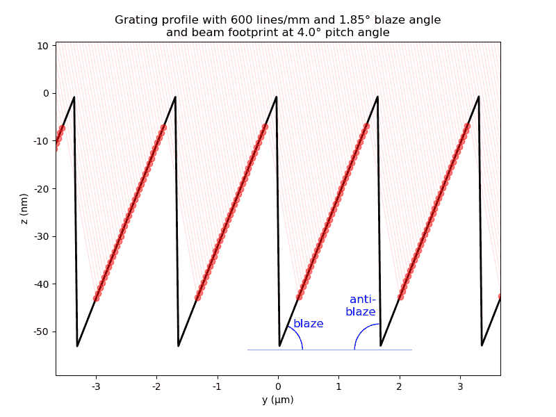
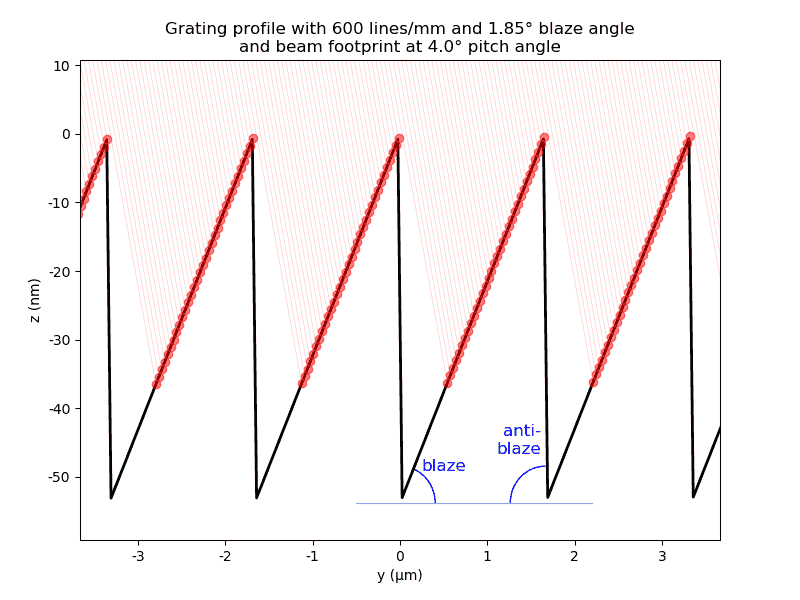
class xrt.backends.raycing.oes.LaminarGrating(OE)

Implements a grating of rectangular profile.

class xrt.backends.raycing.oes.VLSLaminarGrating(OE)

Implements a grating of rectangular profile with variable period.

__init__(*args, **kwargs)

aspect: float

Top-to-period ratio of the groove.

depth: float

Depth of the groove in mm.

For the VLS density, use gratingDensity of the parental class OE with the 1st argument ‘y’ (i.e. along y-axis).

Distorted surfaces

For introducing an error to an ideal surface you must define two methods in your descendant of the OE: local_z_distorted (or local_r_distorted for a parametric surface) and local_n_distorted. The latter method returns two angles d_pitch and d_roll or a 3D vector that will be added to the local normal. See the docstrings of OE.local_n_distorted() and the example ‘Defocusing by a distorted mirror’.

Tests of Optical elements

See the tests here.

Materials

Module materials defines atomic and material properties related to x-ray scattering, diffraction and propagation: reflectivity, transmittivity, refractive index, absorption coefficient etc.

xrt.backends.raycing.materials.read_atomic_data(elem)

Reads atomic data from AtomicData.dat file adopted from XOP [XOP]. It has the following data: 0 AtomicRadius[Å] CovalentRadius[Å] AtomicMass BoilingPoint[K] MeltingPoint[K] Density[g/ccm] AtomicVolume CoherentScatteringLength[1E-12cm] IncoherentX-section[barn] Absorption@1.8Å[barn] DebyeTemperature[K] ThermalConductivity[W/cmK]

In read_atomic_data() only the mass is inquired. The user may extend the method to get the other values by simply adding the corresponding array elements to the returned value.

class xrt.backends.raycing.materials.Element

This class serves for accessing the scattering factors f0, f1 and f2 of a chemical element. It can also report other atomic data listed in AtomicData.dat file adopted from XOP [XOP].

__init__(elem=None, table='Chantler')

elem: str or int

The element can be specified by its name (case sensitive) or its ordinal number.

table: str

This parameter is explained in the description of Material.

get_f0(qOver4pi=0)

Calculates f0 for the given qOver4pi.

get_f1f2(E)

Calculates (interpolates) f1 and f2 for the given array E.

read_f0_Kissel()

Reads f0 scattering factors from the tabulation of XOP [XOP]. These were calculated by [Kissel] and then parameterized as [Waasmaier]:

\[f_0\left(\frac{q}{4\pi}\right) = c + \sum_{i=1}^5{a_i\exp\left(-b_i \left(q/(4\pi)\right)^2\right)}\]

where \(q/(4\pi) = \sin{\theta} / \lambda\) and \(a_i\), \(b_i\) and \(c\) are the coefficients tabulated in the file f0_xop.dat.

[Kissel]

L. Kissel, Radiation physics and chemistry 59 (2000) 185-200, http://www-phys.llnl.gov/Research/scattering/RTAB.html

[Waasmaier]

D. Waasmaier & A. Kirfel, Acta Cryst. A51 (1995) 416-413

read_f1f2_vs_E(table)

Reads f1 and f2 scattering factors from the given table at the instantiation time.

class xrt.backends.raycing.materials.Material

Material serves for getting reflectivity, transmittivity, refractive index and absorption coefficient of a material specified by its chemical formula and density. See also predefined materials in modules materials_compounds and materials_elemental.

__init__(elements=None, quantities=None, kind='auto', rho=0, t=None, table='Chantler total', efficiency=None, efficiencyFile=None, name='', refractiveIndex=None)

elements: str or sequence of str

Contains all the constituent elements (symbols)

quantities: None or sequence of floats of length of elements

Coefficients in the chemical formula. If None, the coefficients are all equal to 1.

kind: str

One of ‘mirror’, ‘thin mirror’, ‘plate’, ‘lens’, ‘grating’, ‘FZP’. If ‘auto’, the optical element will decide which material kind to use via its method assign_auto_material_kind().

rho: float

Density in g/cm³.

t: float

Thickness in mm, required only for ‘thin mirror’.

table: str

At the time of instantiation the tabulated scattering factors of each element are read and then interpolated at the requested q value and energy. table can be ‘Henke’ (10 eV < E < 30 keV) [Henke], ‘Chantler’ (11 eV < E < 405 keV) [Chantler] or ‘BrCo’ (30 eV < E < 509 keV) [BrCo].

The tables of f2 factors consider only photoelectric cross-sections. The tabulation by Chantler can optionally have total absorption cross-sections. This option is enabled by table = ‘Chantler total’.

[Henke]

http://henke.lbl.gov/optical_constants/asf.html B.L. Henke, E.M. Gullikson, and J.C. Davis, X-ray interactions: photoabsorption, scattering, transmission, and reflection at E=50-30000 eV, Z=1-92, Atomic Data and Nuclear Data Tables 54 (no.2) (1993) 181-342.

[Chantler]

http://physics.nist.gov/PhysRefData/FFast/Text/cover.html http://physics.nist.gov/PhysRefData/FFast/html/form.html C. T. Chantler, Theoretical Form Factor, Attenuation, and Scattering Tabulation for Z = 1 - 92 from E = 1 - 10 eV to E = 0.4 - 1.0 MeV, J. Phys. Chem. Ref. Data 24 (1995) 71-643.

[BrCo]

http://www.bmsc.washington.edu/scatter/periodic-table.html ftp://ftpa.aps.anl.gov/pub/cross-section_codes/ S. Brennan and P.L. Cowan, A suite of programs for calculating x-ray absorption, reflection and diffraction performance for a variety of materials at arbitrary wavelengths, Rev. Sci. Instrum. 63 (1992) 850-853.

efficiency: sequence of pairs [order, value]

Can be given for kind = ‘grating’ and kind = ‘FZP’. It must correspond to the field order of the OE. It can be given as a constant per diffraction order or as an energy dependence, also per diffraction order. It is a sequence of pairs [order, value], where value is either the efficiency itself or an index in the data file given by efficiencyFile. The data file can either be (1) a pickle file with energy and efficiency arrays as two first dump elements and efficiency shape as (len(energy), orders) or (2) a column file with energy in the leftmost column and the order efficiencies in the next columns. The value is a corresponding array index (zero-based) or a column number (also zero-based, the 0th column is energy). An example of the efficiency calculation can be found in \examples\withRaycing\11_Wave\waveGrating.py.

efficiencyFile: str

See the definition of efficiency.

name: str

Material name. Not used by xrt. Can be used by the user for annotations of graphs or other output purposes. If empty, the name is constructed from the elements and the quantities.

refractiveIndex: float or complex or numpy array or str

Explicitly defines the refractive index of the material. Can be used for the energy ranges not covered by the tables of scattering factors (IR, visible). Can be set as: a) float or complex value, for a constant, energy-independent refractive index. b) a 3-column numpy array containing Energy in eV, real and imaginary parts of the complex refractive index c) filename for an *.xls or CSV table containig same columns as a numpy array in b).

get_absorption_coefficient(E)

Calculates the linear absorption coefficient from the imaginary part of refractive index. E can be an array. The result is in cm^-1.

\[\mu = 2 \Im(n) k.\]

get_amplitude(E, beamInDotNormal, fromVacuum=True)

Calculates amplitude of reflectivity (for ‘mirror’ and ‘thin mirror’) or transmittivity (for ‘plate’ and ‘lens’) [wikiFresnelEq], [Als-Nielsen]. E is energy, beamInDotNormal is cosine of the angle between the incoming beam and the normal (\(\theta_1\) below), both can be scalars or arrays. The interface of the material is assumed to be with vacuum; the direction is given by boolean fromVacuum. Returns a tuple of the amplitudes of s and p polarizations and the absorption coefficient in cm^-1.

\[\begin{split}r_s^{\rm mirror} &= \frac{n_1\cos{\theta_1} - n_2\cos{\theta_2}} {n_1\cos{\theta_1} + n_2\cos{\theta_2}}\\ r_p^{\rm mirror} &= \frac{n_2\cos{\theta_1} - n_1\cos{\theta_2}} {n_2\cos{\theta_1} + n_1\cos{\theta_2}}\\ r_{s,p}^{\rm thin\ mirror} &= r_{s,p}^{\rm mirror}\frac{1 - p^2} {1 - (r_{s,p}^{\rm mirror})^2p^2},\end{split}\]

where the phase factor \(p^2 = \exp(2iEtn_2\cos{\theta_2}/c\hbar)\).

\[\begin{split}t_s^{\rm plate,\ lens} &= 2\frac{n_1\cos{\theta_1}} {n_1\cos{\theta_1} + n_2\cos{\theta_2}}t_f\\ t_p^{\rm plate,\ lens} &= 2\frac{n_1\cos{\theta_1}} {n_2\cos{\theta_1} + n_1\cos{\theta_2}}t_f\\\end{split}\]

where \(t_f = \sqrt{\frac{\Re(n_2n_1)\cos{\theta_2}} {cos{\theta_1}}}/|n_1|\).

[wikiFresnelEq]

http://en.wikipedia.org/wiki/Fresnel_equations .

[Als-Nielsen] (1,2)

Jens Als-Nielsen, Des McMorrow, Elements of Modern X-ray Physics, John Wiley and Sons, 2001.

get_refractive_index(E)

Calculates refractive index at given E. E can be an array.

\[n = 1 - \frac{r_0\lambda^2 N_A \rho}{2\pi M}\sum_i{x_i f_i(0)}\]

where \(r_0\) is the classical electron radius, \(\lambda\) is the wavelength, \(N_A\) is Avogadro’s number, \(\rho\) is the material density, M is molar mass, \(x_i\) are atomic concentrations (coefficients in the chemical formula) and \(f_i(0)\) are the complex atomic scattering factor for the forward scattering.

class xrt.backends.raycing.materials.Multilayer

Multilayer serves for getting reflectivity of a multilayer. The multilayer may have variable thicknesses of the two alternating layers as functions of local x and y and/or as a function of the layer number.

__init__(tLayer=None, tThickness=0.0, bLayer=None, bThickness=0.0, nPairs=0.0, substrate=None, tThicknessLow=0.0, bThicknessLow=0.0, idThickness=0.0, power=2.0, substRoughness=0, substThickness=inf, name='', geom='reflected')

tLayer, bLayer, substrate: instance of Material

The top layer material, the bottom layer material and the substrate material.

tThickness and bThickness: float in Å

The thicknesses of the layers. If the multilayer is depth graded, tThickness and bThickness are at the top and tThicknessLow and bThicknessLow are at the substrate. If you need laterally graded thicknesses, modify get_t_thickness and/or get_b_thickness in a subclass.

power: float

Defines the exponent of the layer thickness power law, if the multilayer is depth graded:

\[d_n = A / (B + n)^{power}.\]

tThicknessLow and bThicknessLow: float

Are ignored (left as zeros) if not depth graded.

nPairs: int

The number of layer pairs.

idThickness: float in Å

RMS thickness \(\sigma_{j,j-1}\) of the interdiffusion/roughness interface.

substThickness: float in Å

Is only relevant in transmission if substrate is present.

geom: str

Either ‘transmitted’ or ‘reflected’.

get_amplitude(E, beamInDotNormal, x=None, y=None, ucl=None)

Calculates amplitude of reflectivity [Als-Nielsen]. E is energy, beamInDotNormal is cosine of the angle between the incoming beam and the normal (\(\theta_0\) below), both can be scalars or arrays. The top interface of the multilayer is assumed to be with vacuum. Returns a tuple of the amplitudes of s and p polarizations.

The calculation starts from the bottommost layer (with index \(N\)). The reflectivity from its top into the adjacent layer (\(N-1\)) is:

\[R_N = \frac{r_{N-1, N} + r_{N, N+1} p_N^2} {1 + r_{N-1, N} r_{N, N+1} p_N^2},\]

where the capital \(R\) denotes the net reflectivity of the layer and the small letters \(r\) denote the interface reflectivity (Fresnel equations):

\[r_{j, j+1} = \frac{Q_j - Q_{j+1}}{Q_j + Q_{j+1}},\]

here \(N+1\) refers to the substrate material and

\[Q_j = \sqrt{Q^2 - 8k^2\delta_j + i8k^2\beta_j}, \quad Q = 2k\sin{\theta_0}\]

and \(\delta_j\) and \(\beta_j\) are parts of the refractive index \(n_j = 1 - \delta_j + i\beta_j\). The phase factor \(p_j^2\) is \(\exp(i\Delta_j Q_j)\), \(\Delta_j\) being the layer thickness. The calculation proceeds recursively upwards by layers as

\[R_j = \frac{r_{j-1, j} + R_{j+1} p_j^2} {1 + r_{j-1, j} R_{j+1} p_j^2},\]

until \(R_1\) is reached, where the 0th layer is vacuum and \(Q_0 = Q\).

If the interdiffusion thickness is not zero, the reflectivity at each interface is attenuated by a factor of \(exp(-2k_{j,z}k_{j-1,z}\sigma^{2}_{j,j-1})\), where \(k_{j,z}\) is longitudinal component of the wave vector in j-th layer [Nevot-Croce].

The above formulas refer to s polarization. The p part differs at the interface:

\[r^p_{j, j+1} = \frac{Q_j\frac{n_{j+1}}{n_j} - Q_{j+1}\frac{n_{j}}{n_{j+1}}}{Q_j\frac{n_{j+1}}{n_j} + Q_{j+1}\frac{n_{j}}{n_{j+1}}}\]

and thus the p polarization part requires a separate recursive chain.

In transmission, the recursion is the following:

\[T_{N+1} = \frac{t_{N, N+1}t_{N+1, N+2}p_{N+1}} {1 + r_{N, N+1} r_{N+1, N+2} p_N^2}, \quad T_j = \frac{T_{j+1}t_{j-1, j}p_j}{1 + r_{j-1, j} R_{j+1} p_j^2},\]

where the layer \(N+2\) is vacuum and the interface transmittivities for the two polarizations are equal to:

\[t^s_{j, j+1} = \frac{2Q_j}{Q_j + Q_{j+1}}, \quad t^p_{j, j+1} = \frac{2Q_j\frac{n_{j+1}}{n_j}} {Q_j\frac{n_{j+1}}{n_j} + Q_{j+1}\frac{n_{j}}{n_{j+1}}}\]

[Nevot-Croce]

L. Nevot and P. Croce, Rev. Phys. Appl. 15, (1980) 761

get_b_thickness(x, y, iPair)

The bottom (the lower in the period pair) layer thickness in Å as a function of local coordinates x and y and the index (zero at vacuum) of the period pair.

For parametric surfaces, the x and y local coordinates are assumed to be s and phi of the parametric representation.

get_dtheta_symmetric_Bragg(E, order=1)

The angle correction for the symmetric Bragg case:

\[\delta\theta = \theta_B - \arcsin(\sqrt{m^2\lambda^2 + 8 d^2 \overline\delta} / 2d),\]

where \(\overline\delta\) is the period-averaged real part of the refractive index.

get_t_thickness(x, y, iPair)

The top (the upper in the period pair) layer thickness in Å as a function of local coordinates x and y and the index (zero at vacuum) of the period pair.

For parametric surfaces, the x and y local coordinates are assumed to be s and phi of the parametric representation.

class xrt.backends.raycing.materials.Coated

Derivative class from Mutilayer with a single reflective layer on a substrate.

__init__(*args, **kwargs)

coating, substrate: instance of Material

Material of the mirror coating layer, and the substrate material.

cThickness: float

The thicknesses of mirror coating in Å.

surfaceRoughness: float

RMS rougness of the mirror surface in Å.

substRoughness: float

RMS rougness of the mirror substrate in Å.

class xrt.backends.raycing.materials.Crystal(Material)

The parent class for crystals. The descendants must define get_structure_factor(). Crystal gives reflectivity and transmittivity of a crystal in Bragg and Laue cases.

__init__(hkl=[1, 1, 1], d=0, V=None, elements='Si', quantities=None, rho=0, t=None, factDW=1.0, geom='Bragg reflected', table='Chantler total', name='', volumetricDiffraction=False, useTT=False, nu=None, mosaicity=0)

hkl: sequence

hkl indices.

d: float

Interatomic spacing in Å.

V: float

Unit cell volume in ų. If not given, is calculated from d assuming a cubic symmetry.

factDW: float

Debye-Waller factor applied to the structure factor.

geom: str

The 1st word is either ‘Bragg’ or ‘Laue’, the 2nd word is either ‘transmitted’ or ‘reflected’ or ‘Fresnel’ (the optical element must then provide local_g method that gives the grating vector).

table: str

This parameter is explained in the description of the parent class Material.

volumetricDiffraction: bool

By default the diffracted ray originates in the point of incidence on the surface of the crystal in both Bragg and Laue case. When volumetricDiffraction is enabled, the point of diffraction is generated randomly along the transmitted beam path, effectively broadening the meridional beam profile in plain Laue crystal. If the crystal is bent, local deformation of the diffracting plane is taken into account, creating the polychromatic focusing effect.

useTT: bool

Specifies whether the reflectivity is calculated by analytical formula (useTT is False) or by solution of the Takagi-Taupin equations (when useTT is True). The latter case is based on PyTTE code [PyTTE1] [PyTTE2] that was adapted to running the calculations on GPUs.

[PyTTE1] (1,2)

https://github.com/aripekka/pyTTE

[PyTTE2]

A.-P. Honkanen, S. Huotari, IUCrJ 8 (2021) 102-115. doi:10.1107/S2052252520014165

Warning

You need a good graphics card to run these calculations! The corresponding optical element, that utilizes the present crystal material class, must specify targetOpenCL (typically, ‘auto’) and precisionOpenCL (in Bragg cases ‘float32’ is typically sufficient and ‘float64’ is typically needed in Laue cases).

nu: float

Poisson’s ratio. Can be used for calculation of reflectivity in bent isotropic crystals with [PyTTE1]. Not required for plain crystals or for crystals with predefined compliance matrix, see materials_crystals. If provided, overrides existing compliance matrix.

mosaicity: float, radians

The sigma of the normal distribution of the crystallite normals.

xrt follows the concept of mosaic crystals from [SanchezDelRioMosaic]. This concept has three main parts: (i) a random distribution of the crystallite normals results in a distribution in the reflected directions, (ii) the secondary extinction results in a mean free path distribution of the new ray origins and (iii) the reflectivity is calculated following the work [BaconLowde].

In the above stage (ii), the impact points are sampled according to the secondary extinction distribution. For a thin crystal (when t is specified) those rays that go over the crystal thickness retain the original incoming direction and their x, y, z coordinates (the ray heads) are put on the back crystal surface. These rays are also attenuated by the mosaic crystal. Note again that the impact points do not lie on the front crystal surface, so to plot them in a 2D XY plot becomes useless. You can still plot them as YZ or XZ to study the secondary extinction depth. The remaining rays (those sampled within the crystal depth) get reflected and also attenuated depending on the penetration depth.

Note

The amplitude calculation in the mosaic case is implemented only in the reflection geometry. The transmitted beam can still be studied by ray-tracing as we split the beam in our modeling of secondary extinction, see the previous paragraph.

Note

The mosaicity is assumed large compared with the Darwin width. Therefore, there is no continuous transition mosaic-to-perfect crystal at a continuously reduced mosaicity parameter.

See the tests here.

[SanchezDelRioMosaic]

M. Sánchez del Río et al., Rev. Sci. Instrum. 63 (1992) 932.

[BaconLowde]

G. E. Bacon and R. D. Lowde, Acta Crystallogr. 1, (1948) 303.

get_Darwin_width(E, b=1.0, polarization='s')

Calculates the Darwin width as

\[2\delta = |C|\sqrt{\chi_h\chi_{\overline{h}} / b}/\sin{2\theta}\]

get_amplitude(E, beamInDotNormal, beamOutDotNormal=None, beamInDotHNormal=None, xd=None, yd=None)

Calculates complex amplitude reflectivity and transmittivity for s- and p-polarizations (\(\gamma = s, p\)) in Bragg and Laue cases for the crystal of thickness L, based upon Belyakov & Dmitrienko [BD]:

\[\begin{split}R_{\gamma}^{\rm Bragg} &= \chi_{\vec{H}}C_{\gamma}\left(\alpha + i\Delta_{\gamma}\cot{l_{\gamma}}\right)^{-1}|b|^{-\frac{1}{2}}\\ T_{\gamma}^{\rm Bragg} &= \left(\cos{l{_\gamma}} - i\alpha\Delta {_\gamma}^{-1}\sin{l_{\gamma}}\right)^{-1} \exp{\left(i\vec{\kappa}_0^2 L (\chi_0 - \alpha b) (2\vec{\kappa}_0\vec{s})^{-1}\right)}\\ R_{\gamma}^{\rm Laue} &= \chi_{\vec{H}}C_{\gamma} \Delta_{\gamma}^{-1}\sin{l_{\gamma}}\exp{\left(i\vec{\kappa}_0^2 L (\chi_0 - \alpha b) (2\vec{\kappa}_0\vec{s})^{-1}\right)} |b|^{-\frac{1}{2}}\\ T_{\gamma}^{\rm Laue} &= \left(\cos{l_{\gamma}} + i\alpha \Delta_{\gamma}^{-1}\sin{l_{\gamma}}\right) \exp{\left(i\vec{\kappa}_0^2 L (\chi_0 - \alpha b) (2\vec{\kappa}_0\vec{s})^{-1}\right)}\end{split}\]

where

\[\begin{split}\alpha &= \frac{\vec{H}^2 + 2\vec{\kappa}_0\vec{H}} {2\vec{\kappa}_0^2}+\frac{\chi_0(1-b)}{2b}\\ \Delta_{\gamma} &= \left(\alpha^2 +\frac{C_{\gamma}^2\chi_{\vec{H}} \chi_{\overline{\vec{H}}}}{b}\right)^{\frac{1}{2}}\\ l_{\gamma} &= \frac{\Delta_{\gamma}\vec{\kappa}_0^2L} {2\vec{\kappa}_{\vec{H}}\vec{s}}\\ b &= \frac{\vec{\kappa}_0\vec{s}}{\vec{\kappa}_{\vec{H}}\vec{s}}\\ C_s &= 1, \quad C_p = \cos{2\theta_B}\end{split}\]

In the case of thick crystal in Bragg geometry:

\[R_{\gamma}^{\rm Bragg} = \frac{\chi_{\vec{H}} C_{\gamma}} {\alpha\pm\Delta_{\gamma}}|b|^{-\frac{1}{2}}\]

with the sign in the denominator that gives the smaller modulus of \(R_\gamma\).

\(\chi_{\vec{H}}\) is the Fourier harmonic of the x-ray susceptibility, and \(\vec{H}\) is the reciprocal lattice vector of the crystal. \(\vec{\kappa}_0\) and \(\vec{\kappa}_{\vec{H}}\) are the wave vectors of the direct and diffracted waves. \(\chi_{\vec{H}}\) is calculated as:

\[\chi_{\vec{H}} = - \frac{r_0\lambda^2}{\pi V}F_{\vec{H}},\]

where \(r_e = e^2 / mc^2\) is the classical radius of the electron, \(\lambda\) is the wavelength, V is the volume of the unit cell.

Notice \(|b|^{-\frac{1}{2}}\) added to the formulas of Belyakov & Dmitrienko in the cases of Bragg and Laue reflections. This is needed because ray tracing deals not with wave fields but with rays and therefore not with intensities (i.e. per cross-section) but with flux.

[BD]

V. A. Belyakov and V. E. Dmitrienko, Polarization phenomena in x-ray optics, Uspekhi Fiz. Nauk. 158 (1989) 679–721, Sov. Phys. Usp. 32 (1989) 697–719.

xd and yd are local coordinates of the corresponding optical element. If they are not None and crystal’s get_d method exists, the d spacing is given by the get_d method, otherwise it equals to self.d. In a parametric representation, xd and yd are the same parametric coordinates used in local_r and local_n` methods of the corresponding optical element.

get_amplitude_pytte(E, beamInDotNormal, beamOutDotNormal=None, beamInDotHNormal=None, xd=None, yd=None, alphaAsym=None, Ry=None, Rx=None, ucl=None, tolerance=1e-06, maxSteps=10000000.0, autoLimits=True, signal=None)

Calculates complex amplitude reflectivity for s- and p-polarizations (\(\gamma = s, p\)) in Bragg and Laue cases, based on modified PyTTE code

alphaAsymm: float

Angle of asymmetry in radians.

Ry: float

Meridional radius of curvature in mm. Positive for concave bend.

Rx: float

Sagittal radius of curvature in mm. Positive for concave bend.

ucl:

instance of XRT_CL class, defines the OpenCL device and precision of calculation. Calculations should run fine in single precision, float32. See XRT_CL.

tolerance: float

Precision tolerance for RK adaptive step algorithm.

maxSteps: int

Emergency exit to avoid kernel freezing if the step gets too small.

autoLimits: bool

If True, the algorithm will try to automatically determine the angular range where reflectivity will be calculated by numeric integration. Useful for ray-tracing applications where angle of incidence can be too far from Bragg condition, and integration might take unnesessarily long time.

get_dtheta(E, alpha=None)

The angle correction for the general asymmetric case:

\[\begin{split}\delta\theta = \frac{\mp \gamma_0 \pm \sqrt{\gamma_0^2 \mp (\gamma_0 - \gamma_h) \sqrt{1 - \gamma_0^2} \chi_0 / \sin{2\theta_B}}}{\sqrt{1 - \gamma_0^2}}\\\end{split}\]

where \(\gamma_0 = \sin(\theta_B + \alpha)\), \(\gamma_h = \mp \sin(\theta_B - \alpha)\) and the upper sign is for Bragg and the lower sign is for Laue geometry.

get_dtheta_regular(E, alpha=None)

The angle correction for the general asymmetric case in its simpler version:

\[\begin{split}\delta\theta = (1 - b)/2 \cdot \chi_0 / \sin{2\theta_B}\\ |b| = \sin(\theta_B + \alpha) / \sin(\theta_B - \alpha)\end{split}\]

For the symmetric Bragg b = -1 and for the symmetric Laue b = +1.

get_dtheta_symmetric_Bragg(E)

The angle correction for the symmetric Bragg case:

\[\delta\theta = \chi_0 / \sin{2\theta_B}\]

get_refractive_correction(E, beamInDotNormal=None, alpha=None)

The difference in the glancing angle of incidence for incident and exit waves, Eqs. (2.152) and (2.112) in [Shvydko_XRO]:

\[\theta_c - \theta'_c = \frac{w_H^{(s)}}{2} \left(b - \frac{1}{b} \right) \tan{\theta_c}\]

Note

Not valid close to backscattering.

[Shvydko_XRO]

Yu. Shvyd’ko, X-Ray Optics High-Energy-Resolution Applications, Springer-Verlag Berlin Heidelberg, 2004.

class xrt.backends.raycing.materials.CrystalFcc(Crystal)

A derivative class from Crystal that defines the structure factor for an fcc crystal as:

\[\begin{split}F_{hkl}^{fcc} = f \times \left\{ \begin{array}{rl} 4 &\mbox{if $h,k,l$ are all even or all odd} \\ 0 &\mbox{ otherwise} \end{array} \right.\end{split}\]

class xrt.backends.raycing.materials.CrystalDiamond(CrystalFcc)

A derivative class from Crystal that defines the structure factor for a diamond-like crystal as:

\[F_{hkl}^{\rm diamond} = F_{hkl}^{fcc}\left(1 + e^{i\frac{\pi}{2} (h + k + l)}\right).\]

class xrt.backends.raycing.materials.CrystalSi(CrystalDiamond)

A derivative class from CrystalDiamond that defines the crystal d-spacing as a function of temperature.

__init__(*args, **kwargs)

tK: float

Temperature in Kelvin.

hkl: sequence

hkl indices.

dl_l(t=None)

Calculates the crystal elongation at temperature t. Uses the parameterization from [Swenson]. Less than 1% error; the reference temperature is 19.9C; data is in units of unitless; t must be in degrees Kelvin.

[Swenson]

C.A. Swenson, J. Phys. Chem. Ref. Data 12 (1983) 179

get_Bragg_offset(E, Eref)

Calculates the Bragg angle offset due to a mechanical (mounting) misalignment.

E is the calculated energy of a spectrum feature, typically the edge position.

Eref is the tabulated position of the same feature.

get_a()

Gives the lattice parameter.

class xrt.backends.raycing.materials.CrystalFromCell(Crystal)

CrystalFromCell builds a crystal from cell parameters and atomic positions which can be found e.g. in Crystals.dat of XOP [XOP] or xraylib. See also predefined crystals in module materials_crystals.

Examples:

>>> xtalQu = rm.CrystalFromCell(
>>>     'alphaQuartz', (1, 0, 2), a=4.91304, c=5.40463, gamma=120,
>>>     atoms=[14]*3 + [8]*6,
>>>     atomsXYZ=[[0.4697, 0., 0.],
>>>               [-0.4697, -0.4697, 1./3],
>>>               [0., 0.4697, 2./3],
>>>               [0.4125, 0.2662, 0.1188],
>>>               [-0.1463, -0.4125, 0.4521],
>>>               [-0.2662, 0.1463, -0.2145],
>>>               [0.1463, -0.2662, -0.1188],
>>>               [-0.4125, -0.1463, 0.2145],
>>>               [0.2662, 0.4125, 0.5479]])
>>>
>>> xtalGr = rm.CrystalFromCell(
>>>     'graphite', (0, 0, 2), a=2.456, c=6.696, gamma=120,
>>>     atoms=[6]*4, atomsXYZ=[[0., 0., 0.], [0., 0., 0.5],
>>>                            [1./3, 2./3, 0.], [2./3, 1./3, 0.5]])
>>>
>>> xtalBe = rm.CrystalFromCell(
>>>     'Be', (0, 0, 2), a=2.287, c=3.583, gamma=120,
>>>     atoms=[4]*2, atomsXYZ=[[1./3, 2./3, 0.25], [2./3, 1./3, 0.75]])

__init__(name='', hkl=[1, 1, 1], a=5.43071, b=None, c=None, alpha=90, beta=90, gamma=90, atoms=[14, 14, 14, 14, 14, 14, 14, 14], atomsXYZ=[[0.0, 0.0, 0.0], [0.0, 0.5, 0.5], [0.5, 0.5, 0.0], [0.5, 0.0, 0.5], [0.25, 0.25, 0.25], [0.25, 0.75, 0.75], [0.75, 0.25, 0.75], [0.75, 0.75, 0.25]], atomsFraction=None, tK=0, t=None, factDW=1.0, geom='Bragg reflected', table='Chantler total', nuPoisson=0.0, calcBorrmann=None, useTT=False, mosaicity=0)

name: str

Crystal name. Not used by xrt.

hkl: sequence

hkl indices.

a, b, c: float

Cell parameters in Å. a must be given. b, c, if not given, are equlized to a.

alpha, beta, gamma: float

Cell angles in degrees. If not given, are equal to 90.

atoms: list of str or list of int

List of atoms in the cell given by element Z’s or element names.

atomsXYZ: list of 3-sequences

List of atomic coordinates in cell units.

Note

atoms and atomsXYZ must contain all the atoms, not only the unique ones for a given symmetry group (we do not consider symmetry here). For example, the unit cell of magnetite (Fe3O4) has 3 unique atomic positions and 56 in total; here, all 56 are needed.

atomsFraction: a list of float or None

Atomic fractions. If None, all values are 1.

nuPoisson: float

Poisson’s ratio. Used to calculate the properties of bent crystals.

calcBorrmann: str

Controls the origin of the ray leaving the crystal. Can be ‘None’, ‘uniform’, ‘Bessel’ or ‘TT’. If ‘None’, the point of reflection is located on the surface of incidence. In all other cases the coordinate of the exit point is sampled according to the corresponding distribution: ‘uniform’ is a fast approximation for thick crystals, ‘Bessel’ is exact solution for the flat crystals, ‘TT’ is exact solution of Takagi-Taupin equations for bent and flat crystals (‘TT’ requires targetOpenCL in the Optical Element to be not ‘None’ and useTT in the Crystal to be ‘True’. Not recommended for crystals thicker than 100 µm due to heavy computational load).

useTT: bool

Specifies whether the reflectivity will by calculated by analytical formula or by solution of the Takagi-Taupin equations (so far only for the Laue geometry). Must be set to ‘True’ in order to calculate the reflectivity of bent crystals.

class xrt.backends.raycing.materials.Powder(CrystalFromCell)

A derivative class from CrystalFromCell with randomly distributed atomic plane orientations similar to the real polycrystalline powders. The distribution is uniform in the spherical coordinates, so that the angles of longitudinal and transverse deflection (θ and χ) are both functions of uniformly sampled over [0, 1) variables μ and ν: θ = arccos(μ), χ = 2πν.

The class parameter hkl defines the highest reflex, so that reflectivities are calculated for all possible combinations of indices [mnp], where 0 ≤ m ≤ h, 0 ≤ n ≤ k, 0 ≤ p ≤ l. Only one reflection with the highest amplitude is picked for each incident ray.

Warning

Heavy computational load. Requires OpenCL.

__init__(*args, **kwargs)

chi: 2-list of floats [min, max]

Limits of the χ angle distribution. Zero and π/2 angles correspond to the positive directions of x and z axes.

class xrt.backends.raycing.materials.CrystalHarmonics(CrystalFromCell)

A derivative class from CrystalFromCell, used to calculate multiple orders of the given reflex in one run: n*[hkl], where 1 ≤ n ≤ Nmax i.e. [111], [222], [333] or [220], [440], [660]. Only one harmonic with highest reflectivity is picked for each incident ray. Use this class to estimate the efficiency of higher harmonic rejection schemes.

Warning

Heavy computational load. Requires OpenCL.

__init__(*args, **kwargs)

Nmax: int

Specifies the highest order of reflection to be calculated.

class xrt.backends.raycing.materials.MonoCrystal(CrystalFromCell)

A derivative class from CrystalFromCell, used for calculation of the single crystal diffraction patterns (so far cubic symettries only). Similar to the parent class, parameter hkl defines the cut orientation, whereas Nmax stands for the highest index to consider, i.e. for every ray the code would calculate the range of reflexes from [-Nmax, -Nmax, -Nmax] to [Nmax, Nmax, Nmax] (required amount of reflectivity calculations is therefore 2*(2*Nmax+1)^3 per every ray), but only return one of them regarding their intensities. Brighter reflexes would be selected with higher probability.

Warning

Heavy computational load. Requires OpenCL. Decent GPU highly recommended.

__init__(*args, **kwargs)

Nmax: int

Specifies the highest order of reflection to be calculated.

Predefined Materials

CrystalsCompoundsElemental

The module materials_crystals contains predefined classes for most commonly used crystals. Lattice parameters, atomic positions and references have been semi-automatically parsed from XOP/DABAX [XOP] Crystals.dat. To use a crystal in a script simply import the module and instantiate its class:

import xrt.backends.raycing.materials_crystals as xcryst
myInSbXtal = xcryst.InSb(hkl=(3, 1, 1))  # default hkl=(1, 1, 1)

The crystals inherit from Crystal and can use its methods to calculate diffraction amplitudes, the Darwin width, extinction depth etc.

The following crystal classes are defined in this module (sorted by cell volume in ų), marked in bold are those with available elastic constants:

Be (16.23), Graphite (34.98), Titanium (35.32), Diamond (45.38), Iron (46.31), Copper (47.24), Platinum (60.43), LiF (65.27), Aluminum (66.41), Gold (67.83), LaB6 (71.61), LaB6NIST (71.83), SiC (82.2), AlphaQuartz (113), Si (160.2), GaP (161.9), NaCl (179.4), GaAs (180.7), Ge (181.1), InP (202.1), CsF (216.9), InAs (219.9), GaSb (226.5), KCl (249.2), Sapphire (254.7), AlphaAlumina (254.8), InSb (271.9), LiNbO3 (318.2), PET (324.8), CsCl (345.9), Beryl (657.3), TlAP (855.9), KAP (858.9), RbAP (862.9), KTP (871.3), Muscovite (934.2)

Tests of Materials

See the tests here.

Apertures

Module apertures defines rectangular and round apertures and a set of coplanar rectangular apertures. Rectangular apertures may have one or more defining edges. For example, a simple obstacle, like a beam stop block would have one edge, a block of front-end slits would have two edges at 90 degrees to each other, and a collimator would have all four edges.

The classes have useful methods for getting divergence from the aperture size, for setting divergence (calculating the aperture size given the divergence) and for touching the beam with the aperture, i.e. calculating the minimum aperture size that lets the whole beam through.

class xrt.backends.raycing.apertures.RectangularAperture

Implements an aperture or an obstacle as a combination of straight edges.

__init__(bl=None, name='', center=[0, 0, 0], kind=['left', 'right', 'bottom', 'top'], opening=[-10, 10, -10, 10], x='auto', z='auto', alarmLevel=None)

bl: instance of BeamLine

Container for beamline elements. Optical elements are added to its slits list.

name: str

User-specified name, can be used for diagnostics output.

center: 3-sequence of floats

3D point in global system.

kind: sequence

Any combination of ‘top’, ‘bottom’, ‘left’, ‘right’.

opening: sequence

Distances (with sign according to the local coordinate system) from the blade edges to the aperture center with the length corresponding to kind.

x, z: 3-tuples or ‘auto’.

Normalized 3D vectors in the global system which determine the local x and z axes lying in the aperture plane. If x is ‘auto’, it is horizontal and normal to the beam line. If z is ‘auto’, it is vertical. Both x and z can also be set as instance attributes.

alarmLevel: float or None.

Allowed fraction of number of rays absorbed at the aperture relative to the number of incident rays. If exceeded, an alarm output is printed in the console.

get_divergence(source)

Gets divergences given the blade openings.

prepare_wave(prevOE, nrays, rw=None)

Creates the beam arrays used in wave diffraction calculations. prevOE is the diffracting element: a descendant from OE, RectangularAperture or RoundAperture. nrays of samples are randomly distributed over the slit area.

propagate(beam=None, needNewGlobal=False)

Assigns the “lost” value to beam.state array for the rays intercepted by the aperture. The “lost” value is -self.ordinalNum - 1000.

set_divergence(source, divergence)

Gets the blade openings given divergences. divergence is a sequence corresponding to kind

touch_beam(beam)

Adjusts the aperture (i.e. sets self.opening) so that it touches the beam.

class xrt.backends.raycing.apertures.RoundAperture

Implements a round aperture meant to represent a pipe or a flange.

__init__(bl=None, name='', center=[0, 0, 0], r=1, x='auto', z='auto', alarmLevel=None)

A round aperture aperture.

r is the radius.

x, z: 3-tuples or ‘auto’.

Normalized 3D vectors in the global system which determine the local x and z axes lying in the aperture plane. If x is ‘auto’, it is horizontal and normal to the beam line. If z is ‘auto’, it is vertical. Both x and z can also be set as instance attributes.

get_divergence(source)

Gets the full divergence given the aperture radius.

propagate(beam=None, needNewGlobal=False)

Assigns the “lost” value to beam.state array for the rays intercepted by the aperture. The “lost” value is -self.ordinalNum - 1000.

class xrt.backends.raycing.apertures.RoundBeamStop

Implements a round beamstop. Descends from RoundAperture and has the same parameters.

class xrt.backends.raycing.apertures.DoubleSlit

Implements an aperture or an obstacle with a combination of horizontal and/or vertical edge(s).

__init__(*args, **kwargs)

Same parameters as in RectangularAperture and additionally shadeFraction as a value from 0 to 1.

class xrt.backends.raycing.apertures.PolygonalAperture

Implements an aperture or an obstacle defined as a set of polygon vertices.

__init__(bl=None, name='', center=[0, 0, 0], opening=None, x='auto', z='auto', alarmLevel=None)

bl: instance of BeamLine

Container for beamline elements. Optical elements are added to its slits list.

name: str

User-specified name, can be used for diagnostics output.

center: 3-sequence of floats

3D point in global system.

opening: sequence

Coordinates [(x0, y0),…(xN, yN)] of the polygon vertices.

x, z: 3-tuples or ‘auto’.

Normalized 3D vectors in the global system which determine the local x and z axes lying in the aperture plane. If x is ‘auto’, it is horizontal and normal to the beam line. If z is ‘auto’, it is vertical. Both x and z can also be set as instance attributes.

alarmLevel: float or None.

Allowed fraction of number of rays absorbed at the aperture relative to the number of incident rays. If exceeded, an alarm output is printed in the console.

class xrt.backends.raycing.apertures.GridAperture

Implements a grid of rectangular apertures. See tests/raycing/test_polygonal_aperture.py

__init__(bl=None, name='', center=[0, 0, 0], x='auto', z='auto', alarmLevel=None, dx=0.5, dz=0.5, px=1.0, pz=1.0, nx=7, nz=7)

dx and dz: float

Opening sizes (horizontal and vertical).

px and pz: float

Pitch steps (periods).

nx and nz: int

The number of grid openings, counted from the central hole in -ve and +ve directions, making (2*nx+1)*(2*nz+1) rectangular holes in total.

class xrt.backends.raycing.apertures.SiemensStar

Implements a Siemens Star pattern. See tests/raycing/test_polygonal_aperture.py

__init__(bl=None, name='', center=[0, 0, 0], x='auto', z='auto', alarmLevel=None, nSpokes=9, r=0, rx=0, rz=0, phi0=0, vortex=0, vortexNradial=7)

nSpokes: int

The number of spoke openings.

r or (rx and rz): float

The radius of spokes or ellipse semiaxes.

phi0: float

The angle of rotation of the star. At 0 (default), the center of the top spoke is vertical.

vortex: float

Lets the spokes bend. At =1, they bend by one spoke position.

vortexNradial: int

Used with non-zero vortex. The number of segments in the bent spokes.

Screens

Module screens defines a flat screen and a hemispheric screen that intercept a beam and give its image.

class xrt.backends.raycing.screens.Screen

Flat screen for beam visualization.

__init__(bl=None, name='', center=[0, 0, 0], x='auto', z='auto', compressX=None, compressZ=None)

bl: instance of BeamLine

Container for beamline elements. Optical elements are added to its screens list.

name: str

User-specified name, can be used for diagnostics output.

center: tuple of 3 floats

3D point in the global system.

x, z: 3-sequence or ‘auto’.

Normalized 3D vectors in the global system which determine the local x and z axes lying in the screen plane. If x is ‘auto’, it is horizontal and perpendicular to the beam line. If z is ‘auto’, it is vertical. Both x and z can also be set as instance attributes.

compressX, compressZ: float

Multiplicative compression coefficients for the corresponding axes. Typically are not needed. Can be useful to account for the viewing camera magnification or when the camera sees the screen at an angle.

expose(beam=None, onlyPositivePath=False)

Exposes the screen to the beam. beam is in global system, the returned beam is in local system of the screen and represents the desired image.

prepare_wave(prevOE, dim1, dim2, dy=0, rw=None, condition=None)

Creates the beam arrays used in wave diffraction calculations. prevOE is the diffracting element: a descendant from OE, RectangularAperture or RoundAperture. dim1 and dim2 are x and z arrays for a flat screen or phi and theta arrays for a hemispheric screen. The two arrays are generally of different 1D shapes. They are used to create a 2D mesh by meshgrid.

condition: a callable defined in the user script with two flattened

meshgrid arrays as inputs and outputs. Can be used to select wave samples. An example:

def condition(d1s, d2s):
    cond = d1s**2 + d2s**2 <= pinholeDia**2 / 4  # in a pinhole
    return d1s[cond], d2s[cond]

class xrt.backends.raycing.screens.HemisphericScreen

Hemispheric screen for beam visualization.

__init__(bl=None, name='', center=[0, 0, 0], R=1000.0, x='auto', z='auto', phiOffset=0, thetaOffset=0)

x, z: 3-tuples or ‘auto’. Normalized 3D vectors in the global system

which determine the local x and z axes of the hemispheric screen. If x (the origin of azimuthal angle φ) is ‘auto’, it coincides with the beamline’s y; if z (the polar axis) is ‘auto’, it is coincides with the beamline’s x. The equator plane is then vertical. The polar angle θ is counted from -π/2 to π/2 with 0 at the equator and π/2 at the polar axis direction. Both x and z can also be set as instance attributes.

R: float

Radius of the hemisphere in mm.

Wave propagation (diffraction)

Time dependent diffraction

We start from the Kirchhoff integral theorem in the general (time-dependent) form [Born & Wolf]:

\[V(r,t)=\frac 1{4\pi }\int _S\left\{[V]\frac{\partial }{\partial n} \left(\frac 1 s\right)-\frac 1{\mathit{cs}}\frac{\partial s}{\partial n}\left[\frac{\partial V}{\partial t}\right]-\frac 1 s\left[\frac {\partial V}{\partial n}\right]\right\}\mathit{dS},\]

where the integration is performed over the selected surface \(S\), \(s\) is the distance between the point \(r\) and the running point on surface \(S\), \(\frac{\partial }{\partial n}\) denotes differentiation along the normal on the surface and the square brackets on \(V\) terms denote retarded values, i.e. the values at time \(t − s/c\). \(V\) is a scalar wave here but can represent any component of the actual electromagnetic wave provided that the observation point is much further than the wave length (surface currents are neglected here). \(V\) depends on position and time; this is something what we do not have in ray tracing. We obtain it from ray characteristics by:

\[V(s,t)=\frac 1{\sqrt{2\pi }}\int U_{\omega }(s)e^{-i\omega t}d\omega,\]

where \(U_{\omega }(s)\) is interpreted as a monochromatic wave field and therefore can be associated with a ray. Here, this is any component of the ray polarization vector times its propagation factor \(e^{ikl(s)}\). Substituting it into the Kirchhoff integral yields \(V(r,t)\). As we visualize the wave fields in space and energy, the obtained \(V(r,t)\) must be back-Fourier transformed to the frequency domain represented by a new re-sampled energy grid:

\[U_{\omega '}(r)=\frac 1{\sqrt{2\pi }}\int V(r,t)e^{i\omega 't} \mathit{dt}.\]

Ingredients:

\[ \begin{align}\begin{aligned}[V]\frac{\partial }{\partial n}\left(\frac 1 s\right)=-\frac{(\hat {\vec s}\cdot \vec n)}{s^2}[V],\\\frac 1{\mathit{cs}}\frac{\partial s}{\partial n}\left[\frac{\partial V}{\partial t}\right]=\frac{ik} s(\hat{\vec s}\cdot \vec n)[V],\\\frac 1 s\left[\frac{\partial V}{\partial n}\right]=\frac{ik} s(\hat {\vec l}\cdot \vec n)[V],\end{aligned}\end{align} \]

where the hatted vectors are unit vectors: \(\hat {\vec l}\) for the incoming direction, \(\hat {\vec s}\) for the outgoing direction, both being variable over the diffracting surface. As \(1/s\ll k\), the 1st term is negligible as compared to the second one.

Finally,

\[U_{\omega '}(r)=\frac{-i}{8\pi ^2\hbar ^2c}\int e^{i(\omega '-\omega)t} \mathit{dt}\int \frac E s\left((\hat{\vec s}\cdot \vec n)+(\hat{\vec l} \cdot \vec n)\right)U_{\omega }(s)e^{ik(l(s)+s)}\mathit{dS}\mathit{dE}.\]

The time-dependent diffraction integral is not yet implemented in xrt.

Stationary diffraction

If the time interval \(t\) is infinite, the forward and back Fourier transforms give unity. The Kirchhoff integral theorem is reduced then to its monochromatic form. In this case the energy of the reconstructed wave is the same as that of the incoming one. We can still use the general equation, where we substitute:

\[\delta (\omega -\omega ')=\frac 1{2\pi }\int e^{i(\omega '-\omega )t} \mathit{dt},\]

which yields:

\[U_{\omega }(r)=-\frac {i k}{4\pi }\int \frac1 s\left((\hat{\vec s}\cdot \vec n)+(\hat{\vec l}\cdot \vec n)\right)U_{\omega }(s)e^{ik(l(s)+s)} \mathit{dS}.\]

How we treat non-monochromaticity? We repeat the sequence of ray-tracing from the source down to the diffracting surface for each energy individually. For synchrotron sources, we also assume a single electron trajectory (so called “filament beam”). This single energy contributes fully coherently into the diffraction integral. Different energies contribute incoherently, i.e. we add their intensities, not amplitudes.

The input field amplitudes can, in principle, be taken from ray-tracing, as it was done by [Shi_Reininger] as \(U_\omega(s) = \sqrt{I_{ray}(s)}\). This has, however, a fundamental difficulty. The notion “intensity” in many ray tracing programs, as in Shadow used in [Shi_Reininger], is different from the physical meaning of intensity: “intensity” in Shadow is a placeholder for reflectivity and transmittivity. The real intensity is represented by the density of rays – this is the way the rays were sampled, while each ray has \(I_{ray}(x, z) = 1\) at the source [shadowGuide], regardless of the intensity profile. Therefore the actual intensity must be reconstructed. We tried to overcome this difficulty by computing the density of rays by (a) histogramming and (b) kernel density estimation [KDE]. However, the easiest approach is to sample the source with uniform ray density (and not proportional to intensity) and to assign to each ray its physical wave amplitudes as s and p projections. In this case we do not have to reconstruct the physical intensity. The uniform ray density is an option for the geometric and synchrotron sources in sources.

Notice that this formulation does not require paraxial propagation and thus xrt is more general than other wave propagation codes. For instance, it can work with gratings and FZPs where the deflection angles may become large.

[Shi_Reininger] (1,2)

X. Shi, R. Reininger, M. Sanchez del Rio & L. Assoufid, A hybrid method for X-ray optics simulation: combining geometric ray-tracing and wavefront propagation, J. Synchrotron Rad. 21 (2014) 669–678.

[shadowGuide]

6. Cerrina, “SHADOW User’s Guide” (1998).

[KDE]

Michael G. Lerner (mglerner) (2013) http://www.mglerner.com/blog/?p=28

Normalization

The amplitude factors in the Kirchhoff integral assure that the diffracted wave has correct intensity and flux. This fact appears to be very handy in calculating the efficiency of a grating or an FZP in a particular diffraction order. Without proper amplitude factors one would need to calculate all the significant orders and renormalize their total flux to the incoming one.

The resulting amplitude is correct provided that the amplitudes on the diffracting surface are properly normalized. The latter are normalized as follows. First, the normalization constant \(X\) is found from the flux integral:

\[F = X^2 \int \left(|E_s|^2 + |E_p|^2 \right) (\hat{\vec l}\cdot \vec n) \mathit{dS}\]

by means of its Monte-Carlo representation:

\[X^2 = \frac{F N }{\sum \left(|E_s|^2 + |E_p|^2 \right) (\hat{\vec l}\cdot \vec n) S} \equiv \frac{F N }{\Sigma(J\angle)S}.\]

The area \(S\) can be calculated by the user or it can be calculated automatically by constructing a convex hull over the impact points of the incoming rays. The voids, as in the case of a grating (shadowed areas) or an FZP (the opaque zones) cannot be calculated by the convex hull and such cases must be carefully considered by the user.

With the above normalization factors, the Kirchhoff integral calculated by Monte-Carlo sampling gives the polarization components \(E_s\) and \(E_p\) as (\(\gamma = s, p\)):

\[E_\gamma(r) = \frac{\sum K(r, s) E_\gamma(s) X S}{N} = \sum{K(r, s) E_\gamma(s)} \sqrt{\frac{F S} {\Sigma(J\angle) N}}.\]

Finally, the Kirchhoff intensity \(\left(|E_s|^2 + |E_p|^2\right)(r)\) must be integrated over the screen area to give the flux.

Note

The above normalization steps are automatically done inside diffract().

Sequential propagation

In order to continue the propagation of a diffracted field to the next optical element, not only the field distribution but also local propagation directions are needed, regardless how the radiation is supposed to be propagated further downstream: as rays or as a wave. The directions are given by the gradient applied to the field amplitude. Because \(1/s\ll k\) (validity condition for the Kirchhoff integral), the by far most significant contribution to the gradient is from the exponent function, while the gradient of the pre-exponent factor is neglected. The new wave directions are thus given by a Kirchhoff-like integral:

\[{\vec \nabla } U_{\omega }(r) = \frac {k^2}{4\pi } \int \frac {\hat{\vec s}} s \left((\hat{\vec s}\cdot \vec n)+(\hat{\vec l}\cdot \vec n)\right) U_{\omega }(s)e^{ik(l(s)+s)} \mathit{dS}.\]

The resulted vector is complex valued. Taking the real part is not always correct as the vector components may happen to be (almost) purely imaginary. Our solution is to multiply the vector components by a conjugate phase factor of the largest vector component and only then to take the real part.

The correctness of this approach to calculating the local wave directions can be verified as follows. We first calculate the field distribution on a flat screen, together with the local directions. The wave front, as the surface normal to these directions, is calculated by linear integrals of the corresponding angular projections. The calculated wave front surface is then used as a new screen, where the diffracted wave is supposed to have a constant phase. This is indeed demonstrated in the example applying phase as color axis. The sharp phase distribution is indicative of a true wave front, which in turn justifies the correct local propagation directions.

After having found two polarization components and new directions on the receiving surface, the last step is to reflect or refract the wave samples as rays locally, taking the complex refractive indices for both polarizations. This approach is applicable also to wave propagation regime, as the reflectivity values are purely local to the impact points.

Usage

Warning

You need a good graphics card for running these calculations!

Note

OpenCL platforms/devices can be inspected in xrtQook (‘GPU’ button)

Warning

Long calculation on GPU in Windows may result in the system message “Display driver stopped responding and has recovered” or python RuntimeError: out of resources (yes, it’s about the driver response, not the lack of memory). The solution is to change TdrDelay registry key from the default value of 2 seconds to some hundreds or even thousands. Please refer to https://msdn.microsoft.com/en-us/library/windows/hardware/ff569918(v=vs.85).aspx

Tip

If you plan to utilize xrt on a multi-GPU platform under Linux, we recommend KDE based systems (e.g. Kubuntu). It is enough to install the package fglrx-updates-dev without the complete graphics driver.

In contrast to ray propagation, where passing through an optical element requires only one method (“reflect” for a reflective/refractive surface or “propagate” for a slit), wave propagation in our implementation requires two or three methods:

1. prepare_wave creates points on the receiving surface where the diffraction integral will be calculated. For an optical element or a slit the points are uniformly randomly distributed (therefore reasonable physical limits must be given); for a screen the points are determined by the screen pixels. The returned wave is an instance of class Beam, where the arrays x, y, z are local to the receiving surface.

2. diffract (as imported function from xrt.backends.raycing.waves or as a method of the diffracted beam) takes a beam local to the diffracting surface and calculates the diffraction integrals at the points prepared by prepare_wave. There are five scalar integrals: two for Es and Ep and three for the components of the diffracted direction (see the previous Section). All five integrals are calculated in the coordinates local to the diffracting surface but at the method’s end these are transformed to the local coordinates of the receiving surface (remained in the wave container) and to the global coordinate system (a Beam object returned by diffract).

For slits and screens, the two steps above are sufficient. For an optical element, another step is necessary.

3. reflect method of the optical element is meant to take into account its material properties. The intersection points are already known, as provided by the previous prepare_wave, which can be reported to reflect by noIntersectionSearch=True. Here, reflect takes the beam right before the surface and propagates it to right after it. As a result of such a zero-length travel, the wave gets no additional propagation phase but only a complex-valued reflectivity coefficient and a new propagation direction.

These three methods are enough to describe wave propagation through the complete beamline. The first two methods, prepare_wave and diffract, are split from each other because the diffraction calculations may need several repeats in order to accumulate enough wave samples for attaining dark field at the image periphery. The second method can reside in a loop that will accumulate the complex valued field amplitudes in the same beam arrays defined by the first method. In the supplied examples, prepare_wave for the last screen is done before a loop and all the intermediate diffraction steps are done within that loop.

The quality of the resulting diffraction images is mainly characterized by the blackness of the dark field – the area of expected zero intensity. If the statistics is not sufficient, the dark area is not black, and can even be bright enough to mask the main spot. The contrast depends both on beamline geometry (distances) and on the number of wave field samples (a parameter for prepare_wave). Shorter distances require more samples for the same quality, and for the distances shorter than a few meters one may have to reduce the problem dimensionality by cutting in horizontal or vertical, see the examples of SoftiMAX. In the console output, diffract reports on samples per zone (meaning per Fresnel zone). As a rule of thumb, this figure should be greater than ~10⁴ for a good resulting quality.

OE.prepare_wave(prevOE, nrays, shape='auto', area='auto', rw=None)

Creates the beam arrays used in wave diffraction calculations. prevOE is the diffracting element: a descendant from OE, RectangularAperture or RoundAperture. nrays: if int, specifies the number of randomly distributed samples the surface within self.limPhysX limits; if 2-tuple of ints, specifies (nx, ny) sizes of a uniform mesh of samples.

RectangularAperture.prepare_wave(prevOE, nrays, rw=None)

Creates the beam arrays used in wave diffraction calculations. prevOE is the diffracting element: a descendant from OE, RectangularAperture or RoundAperture. nrays of samples are randomly distributed over the slit area.

Screen.prepare_wave(prevOE, dim1, dim2, dy=0, rw=None, condition=None)

Creates the beam arrays used in wave diffraction calculations. prevOE is the diffracting element: a descendant from OE, RectangularAperture or RoundAperture. dim1 and dim2 are x and z arrays for a flat screen or phi and theta arrays for a hemispheric screen. The two arrays are generally of different 1D shapes. They are used to create a 2D mesh by meshgrid.

condition: a callable defined in the user script with two flattened

meshgrid arrays as inputs and outputs. Can be used to select wave samples. An example:

def condition(d1s, d2s):
    cond = d1s**2 + d2s**2 <= pinholeDia**2 / 4  # in a pinhole
    return d1s[cond], d2s[cond]

xrt.backends.raycing.waves.diffract(oeLocal, wave, targetOpenCL='auto', precisionOpenCL='auto')

Calculates the diffracted field – the amplitudes and the local directions – contained in the wave object. The field on the diffracting surface is given by oeLocal. You can explicitly change OpenCL settings targetOpenCL and precisionOpenCL which are initially set to ‘auto’, see their explanation in xrt.backends.raycing.sources.Undulator.

Coherence signatures

A standard way to define coherence properties is via mutual intensity J (another common name is cross-spectral density) and complex degree of coherence j (DoC, normalized J):

\[\begin{split}J(x_1, y_1, x_2, y_2) \equiv J_{12} = \left<E(x_1, y_1)E^{*}(x_2, y_2)\right>\\ j(x_1, y_1, x_2, y_2) \equiv j_{12} = \frac{J_{12}}{\left(J_{11}J_{22}\right)^{1/2}},\end{split}\]

where the averaging \(\left<\ \right>\) in \(J_{12}\) is over different realizations of filament electron beam (one realization per repeat) and is done for the field components \(E_s\) or \(E_p\) of a field diffracted onto a given \((x, y)\) plane.

Both functions are Hermitian in respect to the exchange of points 1 and 2. There are two common ways of working with them:

1. The horizontal and vertical directions are considered independently by placing the points 1 and 2 on a horizontal or vertical line symmetrically about the optical axis. DoC thus becomes a 1D function dependent on the distance between the points, e.g. as \(j_{12}^{\rm hor}=j(x_1-x_2)\). The intensity distribution is also determined over the same line as a 1D positional function, e.g. as \(I(x)\).

   The widths \(\sigma_x\) and \(\xi_x\) of the distributions \(I(x)\) and \(j(x_1-x_2)\) give the coherent fraction \(\zeta_x\) [Vartanyants2010]

   \[\zeta_x = \left(4\sigma_x^2/\xi_x^2 + 1\right)^{-1/2}.\]

2. The transverse field distribution can be analized integrally (not split into the horizontal and vertical projections) by performing the modal analysis consisting of solving the eigenvalue problem for the matrix \(J^{tr=1}_{12}\) – the matrix \(J_{12}\) normalized to its trace – and doing the standard eigendecomposition:

   \[J^{tr=1}(x_1, y_1, x_2, y_2) = \sum_i{w_i V_i(x_1, y_1)V_i^{+}(x_2, y_2)},\]

   with \(w_i, V_i\) being the ith eigenvalue and eigenvector. \(w_0\) is the fraction of the total flux contained in the 0th (coherent) mode or coherent flux fraction.

   Note

   The matrix \(J_{12}\) is of the size (N_x×N_y)², i.e. squared total pixel size of the image! In the current implementation, we use eigh() method from scipy.linalg, where a feasible image size should not exceed ~100×100 pixels (i.e. ~10⁸ size of \(J_{12}\)).

   Note

   For a fully coherent field \(j_{12}\equiv1\) and \(w_0=1, w_i=0\ \forall i>0\), \(V_0\) being the coherent field.

We also propose a third method that results in the same figures as the second method above.

3. It uses Principal Component Analysis (PCA) applied to the filament images \(E(x, y)\). It consists of the following steps.

   1. Out of r repeats of \(E(x, y)\) build a stacked data matrix \(D\) with N_x×N_y rows and r columns.

   2. The matrix \(J_{12}\) is equal to the product \(DD^{+}\). Instead of solving this huge eigenvalue problem of (N_x×N_y)² size, we solve a typically smaller covariance matrix \(D^{+}D\) of the size r².

   3. The spectra of eigenvalues of matrices \(DD^{+}\) and \(D^{+}D\) are equal, plus zeroes for the bigger matrix.

   4. Their eigenvectors (being eigenmodes \(V_i\) of \(DD^{+}\) and principal component axes \(v_i\) of \(D^{+}D\)) corresponding to the same eigenvalue are transformed to each other with a factor \(D\) or \(D^{+}\): \(\tilde{V}_i = Dv_i\) and \(\tilde{v}_i = D^{+}V_i\), after which transformation they must be additionally normalized (\(\tilde{v}_i\) and \(\tilde{V}_i\) are non-normalized eigenvectors) [the proof is a one line matrix equation].

   Finally, PCA gives exactly the same information as the direct modal analysis (method No 2 above) but is cheaper to calculate by many orders of magnitude.

One can define another measure of coherence as a single number, termed as degree of transverse coherence (DoTC) [Saldin2008]:

\[{\rm DoTC} = \frac{\iiiint |J_{12}|^2 dx_1 dy_1 dx_2 dy_2} {\left[\iint J_{11} dx_1 dy_1\right]^2}\]

[Saldin2008]

E.L. Saldin, E.A. Schneidmiller, M.V. Yurkov, Coherence properties of the radiation from X-ray free electron laser, Opt. Commun. 281 (2008) 1179–88.

[Vartanyants2010]

I.A. Vartanyants and A. Singer, Coherence properties of hard x-ray synchrotron sources and x-ray free-electron lasers, New Journal of Physics 12 (2010) 035004.

We propose to calculate DoTC from the matrix traces [derivation to present in the coming paper] as:

4. 1. DoTC = Tr(J²)/Tr²(J).

   2. DoTC = Tr(D⁺DD⁺D)/Tr²(D⁺D), with the matrix D defined above. The exactly same result as in (a) but obtained with smaller matrices.

Note

A good test for the correctness of the obtained coherent fraction is to find it at various positions on propagating in free space, where the result is expected to be invariant. As appears in the examples of SoftiMAX, the analysis based on DoC never gives an invariant coherent fraction at the scanned positions around the focus. The primary reason for this is the difficulty in the determination of the width of DoC, for the latter typically being a complex-shaped oscillatory curve. In contrast, the modal analysis (the PCA implementation is recommended) and the DoTC give the expected invariance.

Coherence analysis and related plotting

The module coherence has functions for 1D and 2D analysis of coherence and functions for 1D plotting of degree of coherence and and 2D plotting of eigen modes.

The input for the analysis functions is a 3D stack of field images. It can be obtained directly from the undulator class, or from a plot object after several repeats of wave propagation of a filament beam through a beamline. Examples can be found in ...\tests\raycing\test_coherent_fraction_stack.py and in SoftiMAX at MAX IV.

xrt.backends.raycing.coherence.calc_1D_coherent_fraction(U, axisName, axis, p=0)

Calculates 1D degree of coherence (DoC). From its width in respect to the width of intensity distribution also infers the coherent fraction. Both widths are rms. The one of intensity is calculated over the whole axis, the one of DoC is calculated between the first local minima around the center provided that these minima are lower than 0.5.

U: complex valued ndarray, shape(repeats, nx, ny)

3D stack of field images. For a 1D cut along axis, the middle of the other dimension is sliced out.

axis: str, one of ‘x’ or (‘y’ or ‘z’)

Specifies the 1D axis of interest.

p: float, distance to screen

If non-zero, the calculated mutual intensity will be divided by p². This is useful to get proper physical units of the returned intensity if the function is applied directly to the field stacks given by Undulator.multi_electron_stack() that is calculated in angular units.

Returns a tuple of mutual intensity, 1D intensity, 1D DoC, rms width of intensity, rms width of DoC (between the local minima, see above), the position of the minima (only the positive side) and the coherent fraction. This tuple can be fed to the plotting function plot_1D_degree_of_coherence().

xrt.backends.raycing.coherence.plot_1D_degree_of_coherence(data1D, axisName, axis, unit='mm', fig2=None, isIntensityNormalized=False, locLegend='auto')

Provides two plots: a 2D plot of mutual intensity and a 1D plot of intensity and DoC. The latter plot can be shared between the two 1D axes if this function is invoked two times.

data1D: tuple returned by calc_1D_coherent_fraction().

axisName: str, used in labels.

axis: 1D array of abscissa.

unit: str, used in labels.

fig2: matplotlib figure object, if needed for shared plotting of two 1D axes.

isIntensityNormalized: bool, controls the intensity axis label.

locLegend: str, legend location in matplotlib style.

Returns the two figure objects for the user to add suptitles and to export to image files.

Plot examples for one and two 1D curves:

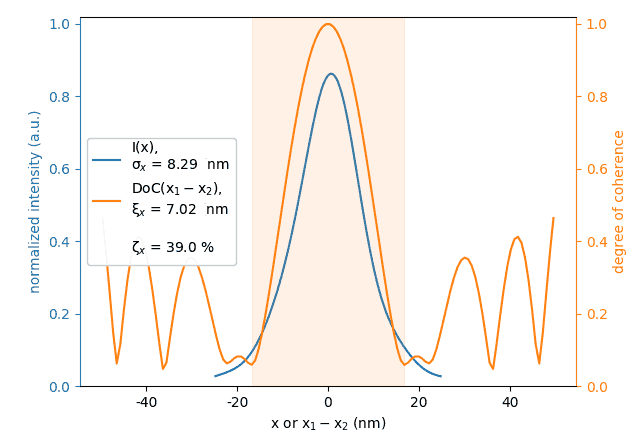
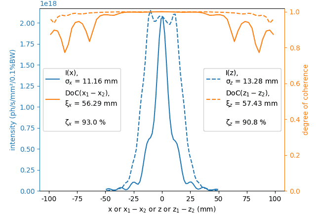
xrt.backends.raycing.coherence.calc_degree_of_transverse_coherence_4D(J)

Calculates DoTC from the mutual intensity J as Tr(J²)/Tr²(J). This function should only be used for demonstration purpose. There is a faster alternative: calc_degree_of_transverse_coherence_PCA().

xrt.backends.raycing.coherence.calc_degree_of_transverse_coherence_PCA(U)

Calculates DoTC from the field stack U. The field images of U are flattened to form the matrix D shaped as (repeats, nx×ny). DoTC = Tr(D⁺DD⁺D)/Tr²(D⁺D), which is equal to the original DoTC for the mutual intensity J: DoTC = Tr(J²)/Tr²(J).

xrt.backends.raycing.coherence.calc_eigen_modes_4D(J, eigenN=4)

Solves the eigenvalue problem for the mutual intensity J. This function should only be used for demonstration purpose. There is a much faster alternative: calc_eigen_modes_PCA().

xrt.backends.raycing.coherence.calc_eigen_modes_PCA(U, eigenN=4, maxRepeats=None, normalize=False)

Solves the PCA problem for the field stack U shaped as (repeats, nx, ny). The field images are flattened to form the matrix D shaped as (repeats, nx×ny). The eigenvalue problem is solved for the matrix D⁺*D*.

Returns a tuple of two arrays: eigenvalues in a 1D array and eigenvectors as columns of a 2D array. This is a much faster and exact replacement of the full eigen mode decomposition by calc_eigen_modes_4D().

eigenN sets the number of returned eigen modes. If None, the number of modes is inferred from the shape of the field stack U and is equal to the number of macroelectrons (repeats). If given as a 2-tuple, eigenN refers to the number of eigenvalues and eigenvectors separately.

if maxRepeats are given, the stack is sliced up to that number. This option is introduced in order not to make the eigenvalue problem too big.

If normalize is True, the eigenvectors are normalized, otherwise they are the PCs of the field stack in the original field units.

xrt.backends.raycing.coherence.plot_eigen_modes(x, y, w, v, xlabel='', ylabel='')

Provides 2D plots of the first 4 eigen modes in the given x and y coordinates. The eigen modes are specified by eigenvalues and eigenvectors w and v returned by calc_eigen_modes_PCA() or calc_eigen_modes_4D().

Plot example:

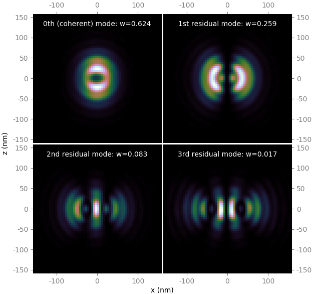
Typical logic for a wave propagation study

1. According to [Wolf], the visibility is not affected by a small bandwidth. It is therefore recommended to first work with strictly monochromatic radiation and check non-monochromaticity at the end.

2. Do a hybrid propagation (waves start somewhere closer to the end) at zero emittance. Put the screen at various positions around the main focus for seeing the depth of focus.

3. Examine the focus and the footprints and decide if vertical and horizontal cuts are necessary (when the dark field does not become black enough at a reasonably high number of wave samples).

4. Run non-zero electron emittance, which spoils both the focal size and the degree of coherence.

5. Try various ways to improve the focus and the degree of coherence: e.g. decrease the exit slit or elongate inter-optics distances.

6. Do hybrid propagation for a finite energy band to study the chromaticity in focus position.

[Wolf]

E. Wolf. Introduction to the theory of coherence and polarization of light. Cambridge University Press, Cambridge, 2007.

Coherent mode decomposition and propagation

The most straightforward way for studying the coherent portion of synchrotron light is first to propagate a large collection of filament beams (or macro-electrons) onto a surface of interest (typically, the focal plane at the sample position) and then perform the modal analysis. The propagation itself may become expensive when optical elements are situated close to each other or when the analysis plane is out of focus. These cases require a large number of wave samples which would allow only a small number of filament beams processed in a reasonable time. In such cases, an inverse approach should be preferred: first do the modal analysis of the source radiation and then propagate the 0th or a few main modes corresponding to the biggest eigenvalues (flux fractions).

In xrt, we calculate a collection of undulator field realizations at the first beamline slit (a front-end slit), transform these fields into modes and save them for the further propagation along the beamline. A selected number of modes, also optionally a selected number of original fields, are prepared for the following three ways of propagation:

1. As waves. The wave samples are sequentially diffracted from the first slit by calculating the Kirchhoff diffraction integral, see Sequential propagation.

2. As hybrid waves. The wave samples at the first slit are treated as rays with the directions projected from the source center (for the modes) or from the filament beam position (for the fields). The beams of these rays can be propagated in ray tracing and then diffracted closer to the end of the beamline. Note that if the beams were propagated as rays down to the image plane, the individual fields would be seen as filament beam dots and the individual modes would be seen as centered dots, i.e. the source would have zero size.

3. As rays. The wave samples at the first slit are propagated backward to the source plane, which gives the field distribution in real space. The field at the first slit is sampled by its intensity; these samples give the ray directions. These beams are suitable for ray traycing down to the image plane. They are not suitable for wave propagation, as the propagation phase of each ray is destroyed by the above resampling procedure.

xrt.backends.raycing.modes.make_and_save_modes(bl, nsamples, nElectrons, nElectronsSave, nModes, fixedEnergy, phaseEsEp=0, output='all', basename='local', limitsOrigin=[])

Produces pickled files of nModes wave modes and nElectronsSave wave fields. The beamline object bl must have at least one aperture; the first of them fill be used to generate nElectrons fields for the eigenmode decomposition. The aperture will be sampled by nsamples wave samples. The fields are normalized such that the intensity sum over the sumples and over nElectrons gives the total flux returned as totalFlux in use_saved(). Note that the total flux is made independent (in average) of nElectrons.

fixedEnergy is photon energy.

phaseEsEp is phase difference between Es and Ep components.

output can be ‘all’ or any combination of words ‘wave’, ‘hybr’, ‘rays’ in one string. The case ‘rays’ can take quite long time for field resampling.

basename is the output file name that will be prepended by the selected ‘wave-’, ‘hybr-’, ‘rays-’ output modes and appended by .pickle.

limitsOrigin as [xmin, xmax, zmin, zmax] must be given for generating ‘rays’.

xrt.backends.raycing.modes.use_saved(what, basename)

Loads the saved modes and fields produced by make_and_save_modes().

what is a string starting with one of ‘wave’, ‘hybr’, ‘rays’ and ending with one of ‘modes’, ‘fields’.

basename is the same parameter used in make_and_save_modes().

Returnes a tuple (savedBeams, wAll, totalFlux), where savedBeams is a list of beam objects corresponding to what. wAll is a list of all eigenvalues (flux weights) of the eigenmode decomposition. totalFlux is described in make_and_save_modes().

See a usage example in /examples/withRaycing/11_Waves/coherentModePropagation.py.

A model case of 5 macro-electrons

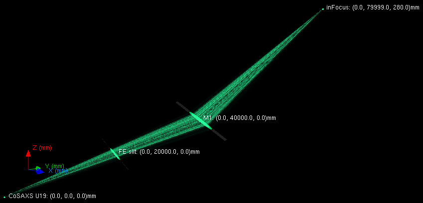
This example was made for the following beamline scheme, where the mirror M1 is an ideal ellipsoid providing 1:1 image of the source.

The eigenmode decomposition at the first slit is accurate within the machine precision, i.e. the total flux summed over all individual fields is equal to the total flux summed over all modes, here down to ~1e-16 relative error. This fact can be proven by comparing the last animation frames of the ‘field’ images vs. ‘mode’ images. This comparison “all fields” vs. “all modes” was the main objective of this “a few macro-electrons” test; in usual studies one would typically need a few thousand macro-electrons and just a small number of modes.

Individual fields

	focus/source	FE slit
rays
hybrid
wave

Coherent modes

	focus/source	FE slit
rays
hybrid
wave

A model case of 5000 macro-electrons

Coherent radiation

The coherent radiation in the 0th mode has a weight (coherent fraction) ≈3.66%. Here it was individually propagated in three different ways:

	focus/source	FE slit
rays
hybrid
wave

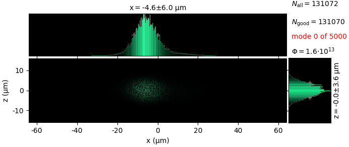
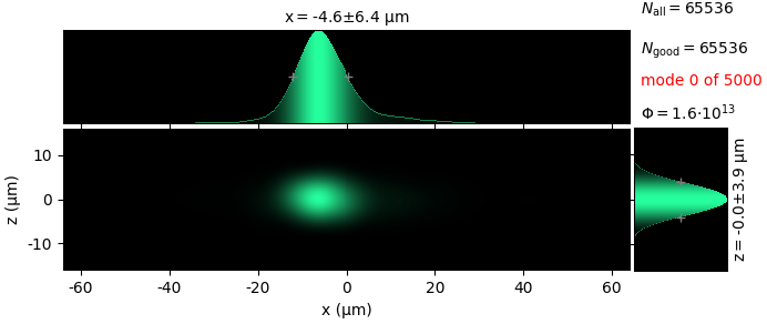
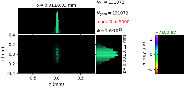
Tests of wave propagation

See the tests here.