Tests of Kirchhoff integral with various Gaussian beams

Find the test module laguerre_gaussian_beam.py, as well as several other tests for raycing backend, in \tests\raycing.

Note

In this section we consider z-axis to be directed along the beamline in order to be compatible with the formulas in their standard notations. Elsewhere in xrt z-axis looks upwards.

Gaussian beam

Gaussian beam at the waist (at \(z=0\)) is defined as

\[u_0(r) = \sqrt{\frac2\pi}\frac1{w_0}\exp\left(-\frac{r^2}{w_0^2}\right),\]

where the pre-exponent factor provides normalization: \(\int{|u|^2dS} = 2\pi\int_0^\infty {|u|^2 rdr} = 1\).

Define

\(z_R \buildrel \text{def}\over = \frac{\pi w_0^2}\lambda\),

\(R \buildrel \text{def}\over = z\left(1+\frac{z_R^2}{z^2}\right)\),

\(w \buildrel \text{def}\over = w_0\sqrt{1+\frac{z^2}{z_R^2}}\).

Gaussian beam at arbitrary z is expressed as:

\[u(r, z) = \sqrt{\frac2\pi}\frac1{w_0}\frac1{1-i\frac{z}{z_R}}\exp \left(-\frac{r^2}{w^2}-\frac{i\pi r^2}{\lambda R}\right),\]

where the exponent can also be rewritten as: \(\exp\left(-\frac{r^2} {w_0^2(1-i\frac{z}{z_R})}\right)\). The pre-exponent factor can also be factored as \(\frac1{1-i\frac{z}{z_R}} = \frac{w_0}w\exp(i\psi)\) with \(\psi= \arctan{\frac{z}{z_R}}=\frac{1}{2i}\log{\frac{1+i\frac{z}{z_R}}{1-i\frac{z} {z_R}}}\).

\(U = u(r, z)\exp\left(-i(kz-\omega t)\right)\) satisfies the wave equation

\[\nabla^2U = \frac{1}{c^2}\frac{\partial^2U}{\partial t^2}.\]

\(u\) can also be obtained by integrating the Gaussian beam waist in a diffraction integral (in our implementation, the Kirchhoff integral):

\[u(x, y, z) = -\frac{ik}{4\pi} \iint_{-\infty}^\infty u_0(x', y') K(x, y, x', y') dx'dy'.\]

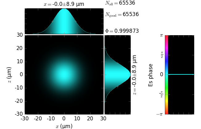
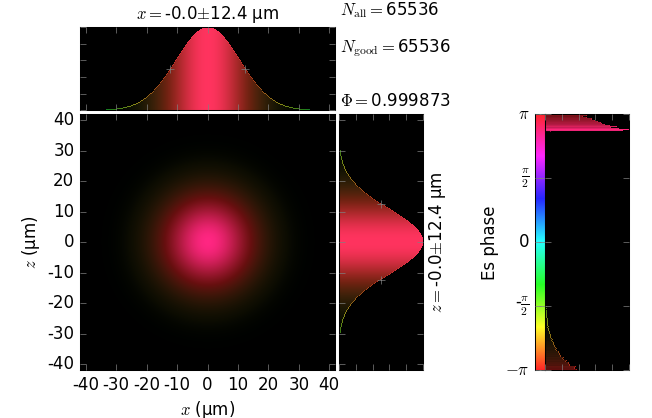
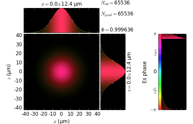
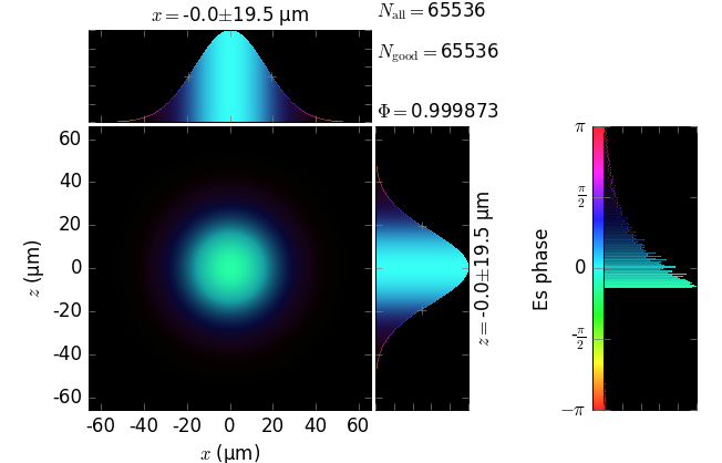
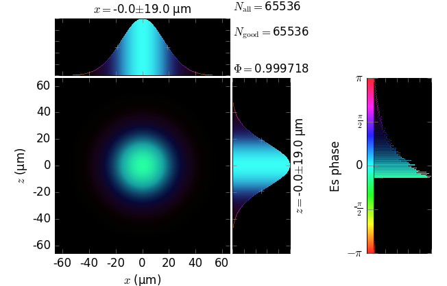
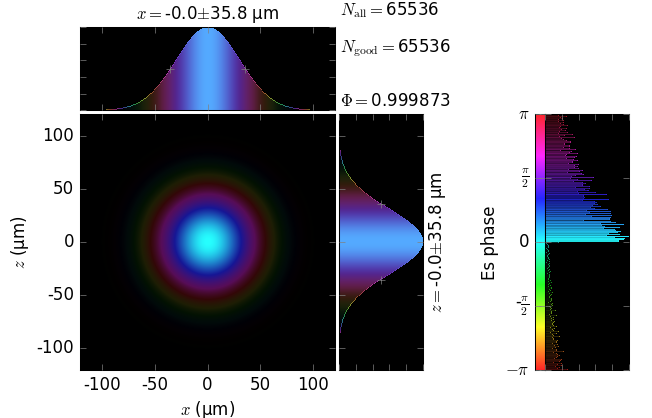
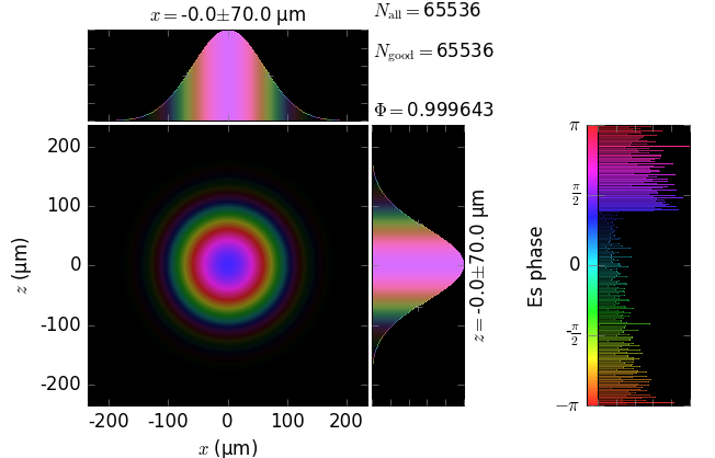
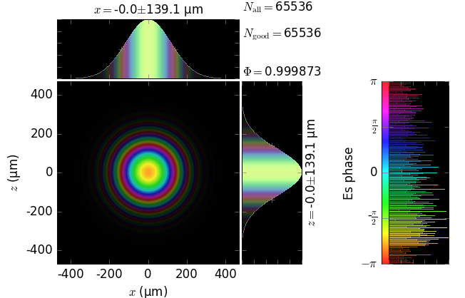
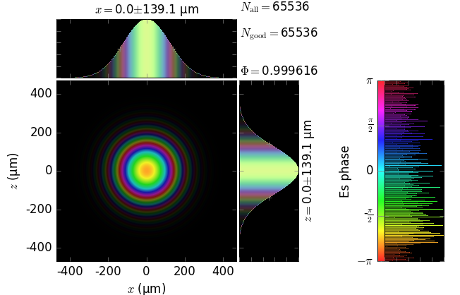
The table below compares Kirchhoff diffraction integrals of a Gaussian waist with analytical solutions. The coloring is by wave phase. Notice equal shape and unity total flux. The Gaussian waist was calculated as GaussianBeam with \(w_0\) = 15 µm:

Gaussian waist (z=0)

Note

The resulting unity flux is not obtained by an ad hoc normalization after the diffraction. This flux is obtained from the diffraction field as is, which demonstrates the correctness of the field amplitude in our implementation of the Kirchhoff integral.

	analytical Gaussian beam	numerical Kirchhoff diffraction
z=5m
z=10m
z=20m
z=40m
z=80m

Laguerre-Gaussian beam

Vortex beams are given by Laguerre-Gaussian modes:

\[u^l_p(r, \phi, z) = u(r, z) \sqrt{\frac{p!}{(p+|l|)!}} \left(\frac{r\sqrt{2}}{w}\right)^{|l|} L^{|l|}_p\left(\frac{2r^2}{w^2}\right) \exp\left(i(|l|+2p)\psi\right)\exp(il\phi).\]

The flux is again normalized to unity.

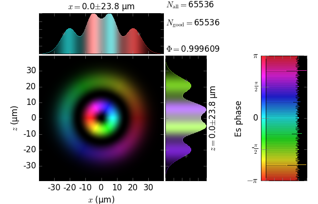
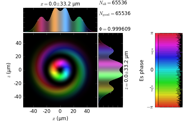
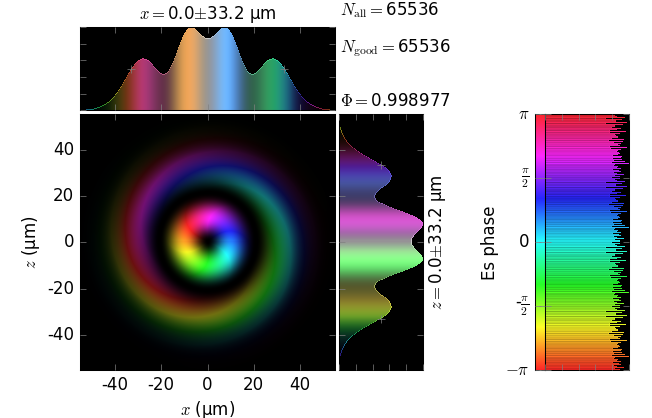
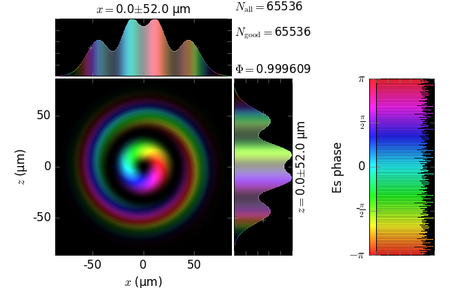
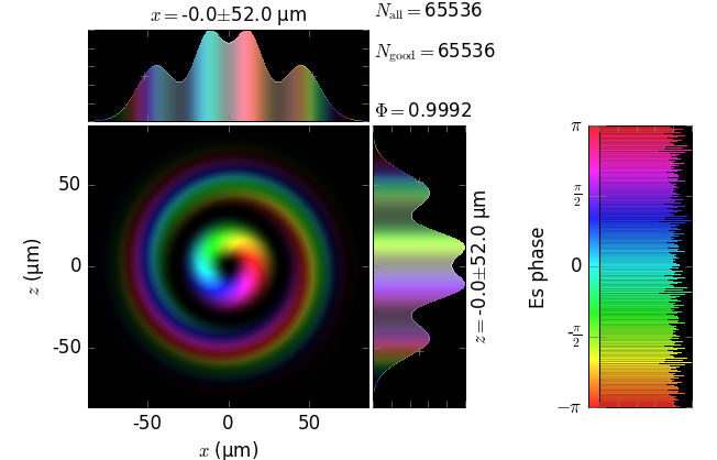
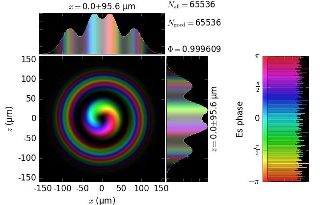
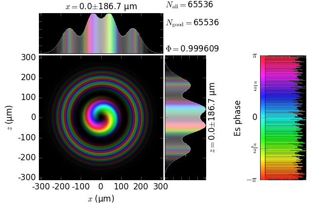
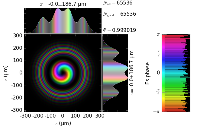
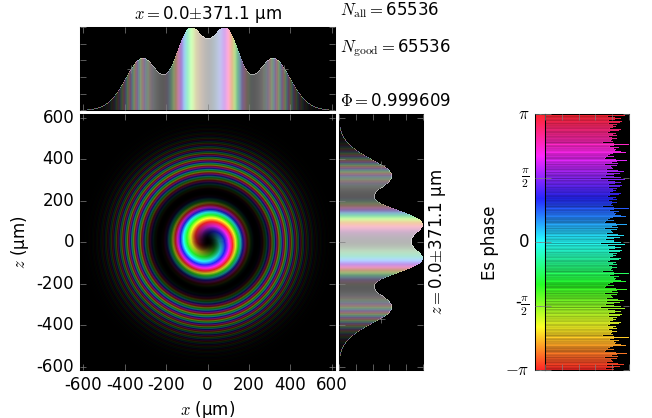
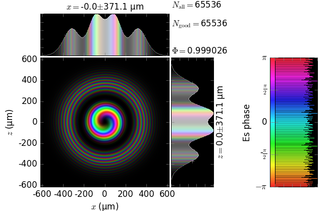
The table below compares Kirchhoff diffraction integrals of a Laguerre-Gaussian waist with analytical solutions. The coloring is by wave phase. Notice equal shape and unity total flux. The Laguerre-Gaussian waist was calculated as LaguerreGaussianBeam with \(w_0\) = 15 µm, \(l\) = 1 and \(p\) = 1:

Laguerre-Gaussian waist (z=0)

Note

The resulting unity flux is not obtained by an ad hoc normalization after the diffraction. This flux is obtained from the diffraction field as is, which demonstrates the correctness of the field amplitude in our implementation of the Kirchhoff integral.

	analytical Laguerre-Gaussian beam	numerical Kirchhoff diffraction
z=5m
z=10m
z=20m
z=40m
z=80m

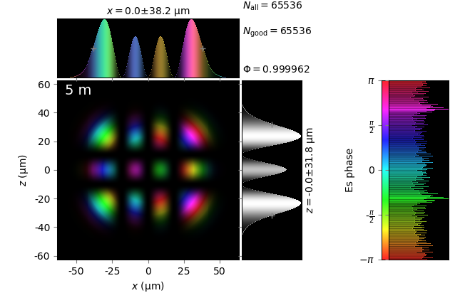
Hermite-Gaussian beam

Higher order modes in rectangular coordinates are given by Hermite-Gaussian modes:

\[u_{mn}(x, y, z) = u(r, z) \frac{1}{\sqrt{2^{m+n}m!n!}} H_m\left(\frac{\sqrt2x}{w}\right) H_n\left(\frac{\sqrt2y}{w}\right) \exp\left(i(m+n)\psi\right),\]

where \(r^2 = x^2 + y^2\). The flux is again normalized to unity.

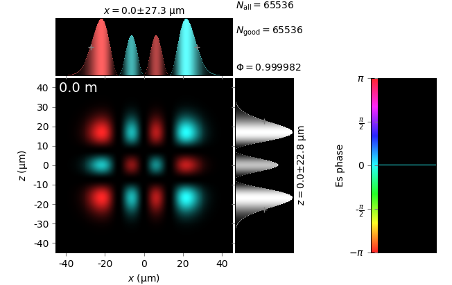
The table below compares Kirchhoff diffraction integrals of a Hermite-Gaussian waist with analytical solutions. The coloring is by wave phase. Notice equal shape and unity total flux. The Hermite-Gaussian waist was calculated as HermiteGaussianBeam with \(w_0\) = 15 µm, \(m\) = 3 and \(n\) = 2:

Hermite-Gaussian waist (z=0)

Note

The resulting unity flux is not obtained by an ad hoc normalization after the diffraction. This flux is obtained from the diffraction field as is, which demonstrates the correctness of the field amplitude in our implementation of the Kirchhoff integral.

	analytical Hermite-Gaussian beam	numerical Kirchhoff diffraction
z=5m
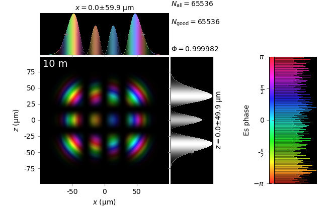
z=10m
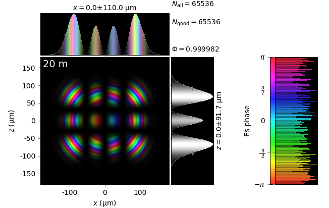
z=20m
z=40m
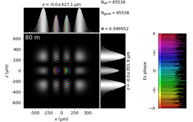
z=80m