Customizing your plots
Module plotter provides classes describing axes and plots, as well as
containers for the accumulated arrays (histograms) for subsequent
pickling/unpickling or for global flux normalization. The module defines
several constants for default plot positions and sizes. The user may want to
modify them in the module or externally as in the xrt_logo.py example.
Note
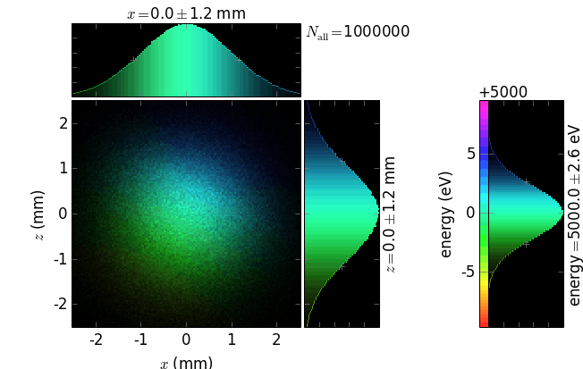
Each plot has a 2D positional histogram, two 1D positional histograms and, typically, a 1D color histogram (e.g. energy).
Warning
The two 1D positional histograms are not calculated from the 2D one!
In other words, the 1D histograms only respect their corresponding limits and not the other dimension’s limits. There can be situations when the 2D image is black because the screen is misplaced but one 1D histogram may still show a beam distribution if in that direction the screen is positioned correctly. This was the reason why the 1D histograms were designed not to be directly dependent on the 2D one – this feature facilitates the troubleshooting of misalignments. On the other hand, this behavior may lead to confusion if a part of the 2D distribution is outside of the visible 2D area. In such cases one or two 1D histograms may show a wider distribution than the one visible on the 2D image. For correcting this behavior, one can mask the beam by apertures or by selecting the physical or optical limits of an optical element.
Tip
If you do not want to create plot windows (e.g. when they are too many or when you run xrt on a remote machine) but only want to save plots, you can use a non-interactive matplotlib backend such as Agg (for PNGs), PDF, SVG or PS:
matplotlib.use('agg')
Importantly, this must be done at the very top of your script, right after import matplotlib and before importing anything else.
The plots can be customized at the time of their creation using many optional
parameters of xrt.plotter.XYCPlot.__init__() constructor.
- class xrt.plotter.XYCPlot(beam=None, rayFlag=(1,), xaxis=None, yaxis=None, caxis=None, aspect='equal', xPos=1, yPos=1, ePos=1, title='', invertColorMap=False, negative=False, fluxKind='total', fluxUnit='auto', fluxFormatStr='auto', contourLevels=None, contourColors=None, contourFmt='%.1f', contourFactor=1.0, saveName=None, persistentName=None, oe=None, raycingParam=0, beamState=None, beamC=None, beamAbsorb=None, showAbsorbed=False, useQtWidget=False)
Container for the accumulated histograms. Besides giving the beam images, this class provides with useful fields like dx, dy, dE (FWHM), cx, cy, cE (centers) and intensity which can be used in scripts for producing scan-like results.
- __init__(beam=None, rayFlag=(1,), xaxis=None, yaxis=None, caxis=None, aspect='equal', xPos=1, yPos=1, ePos=1, title='', invertColorMap=False, negative=False, fluxKind='total', fluxUnit='auto', fluxFormatStr='auto', contourLevels=None, contourColors=None, contourFmt='%.1f', contourFactor=1.0, saveName=None, persistentName=None, oe=None, raycingParam=0, beamState=None, beamC=None, beamAbsorb=None, showAbsorbed=False, useQtWidget=False)
- beam: str
The beam to be visualized.
- In raycing backend:
The key in the dictionary returned by
run_process(). The values of that dictionary are beams (instances ofBeam).- In shadow backend:
The Shadow output file (
star.NN, mirr.NN` orscreen.NNMM). It will also appear in the window caption unless title parameter overrides it.
This parameter is used for the automatic determination of the backend in use with the corresponding meaning of the next two parameters. If beam contains a dot, shadow backend is assumed. Otherwise raycing backend is assumed.
- rayFlag: int or tuple of ints
shadow: 0=lost rays, 1=good rays, 2=all rays. raycing: a tuple of integer ray states: 1=good, 2=out, 3=over, 4=alive (good + out), -NN = dead at oe number NN (numbering starts with 1).
- xaxis, yaxis, caxis: instance of
XYCAxisor None. If None, a default axis is created. If caxis=’category’ and the backend is raycing, then the coloring is given by ray category, the color axis histogram is not displayed and ePos is ignored.
Warning
The axes contain arrays for the accumulation of histograms. If you create the axes outside of the plot constructor then make sure that these are not used for another plot. Otherwise the histograms will be overwritten!
- aspect: str or float
Aspect ratio of the 2D histogram, = ‘equal’, ‘auto’ or numeric value (=x/y). aspect =1 is the same as aspect =’equal’.
- xPos, yPos: int
If non-zero, the corresponding 1D histograms are visible.
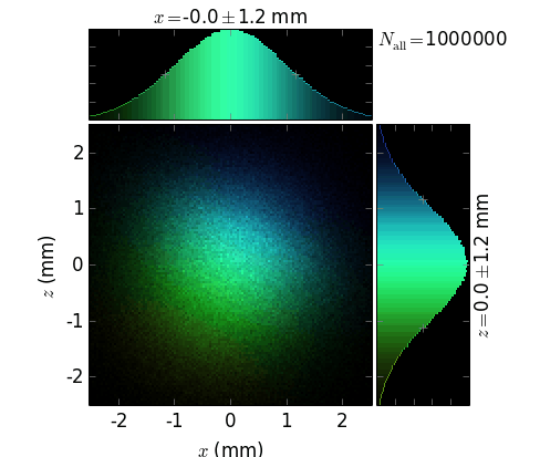
- ePos: int
Flag for specifying the positioning of the color axis histogram:
ePos =1: at the right (default, as usually the diffraction plane is vertical)
ePos =2: at the top (for horizontal diffraction plane)
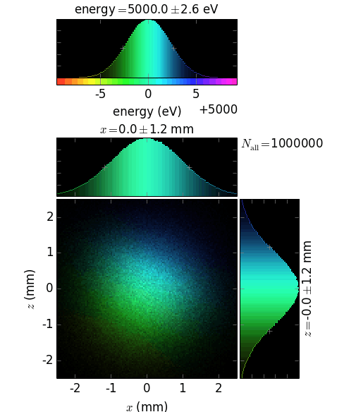
ePos =0: no color axis histogram
- title: str
If non-empty, this string will appear in the window caption, otherwise the beam will be used for this.
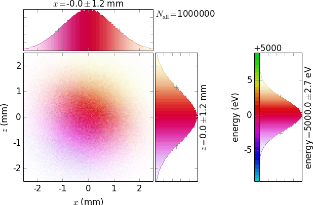
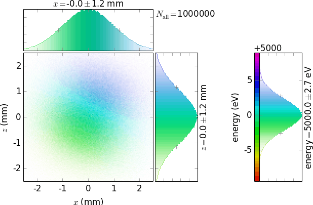
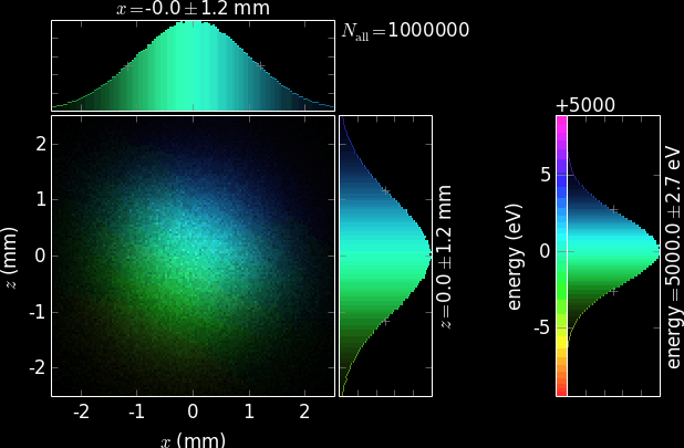
- invertColorMap: bool
Inverts colors in the HSV color map; seen differently, this is a 0.5 circular shift in the color map space. This inversion is useful in combination with negative in order to keep the same energy coloring both for black and for white images.
- negative: bool
Useful for printing in order to save black inks. See also invertColorMap.
=False: black bknd for on-screen presentation
=True: white bknd for paper printing
The following table demonstrates the combinations of invertColorMap and negative:
invertColorMap =False
invertColorMap =True
negative =False
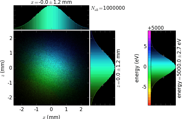
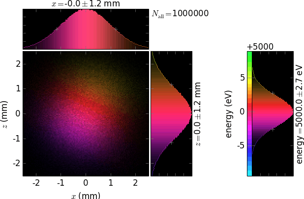
negative =True
Note that negative inverts only the colors of the graphs, not the white global background. Use a common graphical editor to invert the whole picture after doing negative=True:
(such a picture would nicely look on a black journal cover, e.g. on that of Journal of Synchrotron Radiation ;) )
- fluxKind: str
Can begin with ‘s’, ‘p’, ‘+-45’, ‘left-right’, ‘total’, ‘power’, ‘Es’, ‘Ep’ and ‘E’. Specifies what kind of flux to use for the brightness of 2D and for the height of 1D histograms. If it ends with ‘log’, the flux scale is logarithmic.
If starts with ‘E’ then the field amplitude or mutual intensity is considered, not the usual intensity, and accumulated in the 2D histogram or in a 3D stack:
If ends with ‘xx’ or ‘zz’, the corresponding 2D cuts of mutual intensity are accumulated in the main 2D array (the one visible as a 2D histogram). The plot must have equal axes.
If ends with ‘4D’, the complete mutual intensity is calculated and stored in plot.total4D with the shape (xaxis.bins*yaxis.bins, xaxis.bins*yaxis.bins).
Warning
Be cautious with the size of the mutual intensity object, it is four-dimensional!
If ends with ‘PCA’, the field images are stored in plot.field3D with the shape (repeats, xaxis.bins, yaxis.bins) for further Principal Component Analysis.
If without these endings, the field aplitudes are simply summed in the 2D histogram.
- fluxUnit: ‘auto’ or None
If a synchrotron source is used and fluxUnit is ‘auto’, the flux will be displayed as ‘ph/s’ or ‘W’ (if fluxKind == ‘power’). Otherwise the flux is a unitless number of rays times transmittivity | reflectivity.
- fluxFormatStr: str
Format string for representing the flux or power. You can use a representation with powers of ten by utilizing ‘p’ as format specifier, e.g. ‘%.2p’.
- contourLevels: sequence
A sequence of levels on the 2D image for drawing the contours, in [0, 1] range. If None, the contours are not drawn.
- contourColors: sequence or color
A sequence of colors corresponding to contourLevels. A single color value is applied to all the contours. If None, the colors are automatic.
- contourFmt: str
Python format string for contour values.
- contourFactor: float
Is applied to the levels and is useful in combination with contourFmt, e.g. contourFmt = r’%.1f mW/mm$^2$’, contourFactor = 1e3.
- saveName: str or list of str or None
Save file name(s). The file type(s) are given by extensions: png, ps, svg, pdf. Typically, saveName is set outside of the constructor. For example:
filename = 'filt%04imum' %thick #without extension
plot1.saveName = [filename + '.pdf', filename + '.png']
- persistentName: str or None
File name for reading and storing the accumulated histograms and other ancillary data. Ray tracing will resume the histogramming from the state when the persistent file was written. If the file does not exist yet, the histograms are initialized to zeros. The persistent file is rewritten when ray tracing is completed and the number of repeats > 0.
Warning
Be careful when you use it: if you intend to start from zeros, make sure that this option is switched off or the pickle files do not exist! Otherwise you do resume, not really start anew.
if persistentName ends with ‘.mat’, a Matlab file is generated.
- oe: instance of an optical element or None
If supplied, the rectangular or circular areas of the optical surfaces or physical surfaces, if the optical surfaces are not specified, will be overdrawn. Useful with raycing backend for footprint images.
- raycingParam: int
Used together with the oe parameter above for drawing footprint envelopes. If =2, the limits of the second crystal of DCM are taken for drawing the envelope; if =1000, all facets of a diced crystal are displayed.
- beamState: str
Used in raycing backend. If not None, gives another beam that determines the state (good, lost etc.) instead of the state given by beam. This may be used to visualize the incoming beam but use the states of the outgoing beam, so that you see how the beam upstream of the optical element will be masked by it. See the examples for capillaries.
- beamC: str
The same as beamState but refers to colors (when not of ‘category’ type).
Each of the 3 axes: xaxis, yaxis and caxis can be customized using many optional
parameters of xrt.plotter.XYCAxis.__init__() constructor.
- class xrt.plotter.XYCAxis(label='', unit='mm', factor=None, data='auto', limits=None, offset=0, bins=128, ppb=2, density='histogram', invertAxis=False, outline=0.5, fwhmFormatStr='%.1f')
Contains a generic record structure describing each of the 3 axes: X, Y and Color (typ. Energy).
- __init__(label='', unit='mm', factor=None, data='auto', limits=None, offset=0, bins=128, ppb=2, density='histogram', invertAxis=False, outline=0.5, fwhmFormatStr='%.1f')
- label: str
The label of the axis without unit. This label will appear in the axis caption and in the FWHM label.
- unit: str
The unit of the axis which will follow the label in parentheses and appear in the FWHM value
- factor: float
Useful in order to match your axis units with the units of the ray tracing backend. For instance, the shadow length unit is cm. If you want to display the positions as mm: factor=10; if you want to display energy as keV: factor=1e-3. Another usage of factor is to bring the coordinates of the ray tracing backend to the world coordinates. For instance, z-axis in shadow is directed off the OE surface. If the OE is faced upside down, z is directed downwards. In order to display it upside, set minus to factor. if not specified, factor will default to a value that depends on unit. See
def auto_assign_factor().- data: int for shadow, otherwise array-like or function object
- shadow:
zero-based index of columns in the shadow binary files:
0
x
1
y
2
z
3
x’
4
y’
5
z’
6
Ex s polariz
7
Ey s polariz
8
Ez s polariz
9
lost ray flag
10
photon energy
11
ray index
12
optical path
13
phase (s polarization)
14
phase (p polarization)
15
x component of the electromagnetic vector (p polar)
16
y component of the electromagnetic vector (p polar)
17
z component of the electromagnetic vector (p polar)
18
empty
- raycing:
use the following functions (in the table below) or pass your own one. See
raycingfor more functions, e.g. for the polarization properties. Alternatively, you may pass an array of the length of the beam arrays.Note
In Shadow, x’, y’ and z’ are stored ray direction components (often described as direction or divergence). Their direct raycing analogs are a, b and c. For convenience and historical compatibility, raycing auto-assigns x’ and z’ to the slopes a/b and c/b, i.e. to raycing.get_xprime and raycing.get_zprime. The label y’ has no analogous slope definition because b is the reference direction; it is therefore auto-assigned to raycing.get_b.
x
raycing.get_x
y
raycing.get_y
z
raycing.get_z
x’
raycing.get_xprime = a/b
y’
raycing.get_b
z’
raycing.get_zprime = c/b
energy
raycing.get_energy
If data = ‘auto’ then label is searched for “x”, “y”, “z”, “x’”, “y’”, “z’”, “energy” and if one of them is found, data is assigned to the listed above index or function. In raycing backend, automatic assignment first checks whether a corresponding
get_<label>function exists and then falls back to matching labels containing ‘degree (for degree of polarization)’, ‘circular’ (for circular polarization rate), ‘polarization’ and ‘angle’ (for angle of polarization ellipse), ‘ellipse’ or ‘axes’ (for ratio of ellipse axes), ‘phase’, ‘path’, ‘incid’ or ‘theta’ (for incident angle), ‘order’ (for grating diffraction order), and standalone ‘s’, ‘phi’, ‘r’, ‘a’ or ‘b’.- limits: 2-list of floats [min, max]
Axis limits. If None, the limits are taken as
np.minandnp.maxfor the corresponding array acquired after the 1st ray tracing run. If limits == ‘symmetric’, the limits are forced to be symmetric about the origin. Can also be set outside of the constructor as, e.g.:plot1.xaxis.limits = [-15, 15]
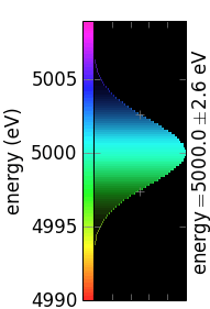
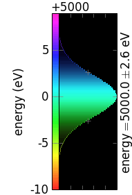
- offset: float
An offset value subtracted from the axis tick labels to be displayed separately. It is useful for the energy axis, where the band width is most frequently much smaller than the central value. Ignored for x and y axes.
no offset
non-zero offset
- bins: int
Number of bins in the corresponding 1D and 2D histograms. See also ppb parameter.
- ppb: int
Screen-pixel-per-bin value. The graph arrangement was optimized for bins * ppb = 256. If your bins and ppb give a very different product, the graphs may look ugly (disproportional) with overlapping tick labels.
- density: ‘histogram’ or ‘kde’
The way the sample density is calculated: by histogram or by kde [KDE].
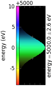
- invertAxis: bool
Inverts the axis direction. Useful for energy axis in energy- dispersive images in order to match the colors of the energy histogram with the colors of the 2D histogram.
- outline: float within [0, 1]
Specifies the minimum brightness of the outline drawn over the 1D histogram. The maximum brightness equals 1 at the maximum of the 1D histogram.
=0
=0.5
=1


- fwhmFormatStr: str
Python format string for the FWHM value, e.g. ‘%.2f’. if None, the FWHM value is not displayed.
Customizing the look of the graphs
The elements of the graphs (fonts, line thickness etc.) can be modified by
editing
the matplotlibrc file.
Alternatively, you can do this “dynamically”, e.g.:
import matplotlib as mpl
mpl.rcParams['font.family'] = 'serif'
mpl.rcParams['font.size'] = 12
mpl.rcParams['axes.linewidth'] = 0.5
The sizes and positions of the graphs are controlled by several constants
specified in xrt. You can either modify them directly in the
module or in your script, like it was done for creating the logo
image (see also logo_xrt.py script in the examples):
import xrt.plotter as xrtp
xrtp.xOrigin2d = 4
xrtp.yOrigin2d = 4
xrtp.height1d = 64
xrtp.heightE1d = 64
xrtp.xspace1dtoE1d = 4
Saving the histogram arrays
The histograms can be saved to and later restored from a persistent file. Doing so is always recommended as this can save you time
afterwards if you decide to change a label or a font size or to make the graphs
negative: you can do this without re-doing ray tracing. Remember, however, that
a new run of the same script will initialize the histograms not from zero but
from the last saved state. You will notice this by the displayed number of rays.
If you want to initialize from zero, just delete the persistent file. Note that
you can run run_ray_tracing() with repeats=0 in order to
re-display the saved plots without starting ray tracing.