Coherent mode decomposition and propagation
The most straightforward way for studying the coherent portion of synchrotron light is first to propagate a large collection of filament beams (or macro-electrons) onto a surface of interest (typically, the focal plane at the sample position) and then perform the modal analysis. The propagation itself may become expensive when optical elements are situated close to each other or when the analysis plane is out of focus. These cases require a large number of wave samples which would allow only a small number of filament beams processed in a reasonable time. In such cases, an inverse approach should be preferred: first do the modal analysis of the source radiation and then propagate the 0th or a few main modes corresponding to the biggest eigenvalues (flux fractions).
In xrt, we calculate a collection of undulator field realizations at the first beamline slit (a front-end slit), transform these fields into modes and save them for the further propagation along the beamline. A selected number of modes, also optionally a selected number of original fields, are prepared for the following three ways of propagation:
As waves. The wave samples are sequentially diffracted from the first slit by calculating the Kirchhoff diffraction integral, see Sequential propagation.
As hybrid waves. The wave samples at the first slit are treated as rays with the directions projected from the source center (for the modes) or from the filament beam position (for the fields). The beams of these rays can be propagated in ray tracing and then diffracted closer to the end of the beamline. Note that if the beams were propagated as rays down to the image plane, the individual fields would be seen as filament beam dots and the individual modes would be seen as centered dots, i.e. the source would have zero size.
As rays. The wave samples at the first slit are propagated backward to the source plane, which gives the field distribution in real space. The field at the first slit is sampled by its intensity; these samples give the ray directions. These beams are suitable for ray traycing down to the image plane. They are not suitable for wave propagation, as the propagation phase of each ray is destroyed by the above resampling procedure.
- xrt.backends.raycing.modes.make_and_save_modes(bl, nsamples, nElectrons, nElectronsSave, nModes, fixedEnergy, phaseEsEp=0, output='all', basename='local', limitsOrigin=[])
Produces pickled files of nModes wave modes and nElectronsSave wave fields. The beamline object bl must have at least one aperture; the first of them fill be used to generate nElectrons fields for the eigenmode decomposition. The aperture will be sampled by nsamples wave samples. The fields are normalized such that the intensity sum over the sumples and over nElectrons gives the total flux returned as totalFlux in use_saved(). Note that the total flux is made independent (in average) of nElectrons.
fixedEnergy is photon energy.
phaseEsEp is phase difference between Es and Ep components.
output can be ‘all’ or any combination of words ‘wave’, ‘hybr’, ‘rays’ in one string. The case ‘rays’ can take quite long time for field resampling.
basename is the output file name that will be prepended by the selected ‘wave-’, ‘hybr-’, ‘rays-’ output modes and appended by .pickle.
limitsOrigin as [xmin, xmax, zmin, zmax] must be given for generating ‘rays’.
- xrt.backends.raycing.modes.use_saved(what, basename)
Loads the saved modes and fields produced by make_and_save_modes().
what is a string starting with one of ‘wave’, ‘hybr’, ‘rays’ and ending with one of ‘modes’, ‘fields’.
basename is the same parameter used in make_and_save_modes().
Returnes a tuple (savedBeams, wAll, totalFlux), where savedBeams is a list of beam objects corresponding to what. wAll is a list of all eigenvalues (flux weights) of the eigenmode decomposition. totalFlux is described in make_and_save_modes().
See a usage example in
/examples/withRaycing/11_Waves/coherentModePropagation.py.
A model case of 5 macro-electrons
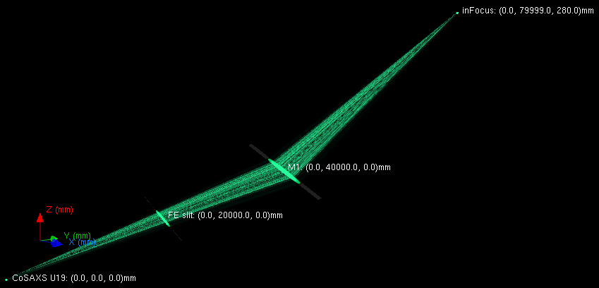
This example was made for the following beamline scheme, where the mirror M1 is an ideal ellipsoid providing 1:1 image of the source.
The eigenmode decomposition at the first slit is accurate within the machine precision, i.e. the total flux summed over all individual fields is equal to the total flux summed over all modes, here down to ~1e-16 relative error. This fact can be proven by comparing the last animation frames of the ‘field’ images vs. ‘mode’ images. This comparison “all fields” vs. “all modes” was the main objective of this “a few macro-electrons” test; in usual studies one would typically need a few thousand macro-electrons and just a small number of modes.
Individual fields
focus/source |
FE slit |
|
|---|---|---|
rays |
||
hybrid |
||
wave |
Coherent modes
focus/source |
FE slit |
|
|---|---|---|
rays |
||
hybrid |
||
wave |
A model case of 5000 macro-electrons
Coherent radiation
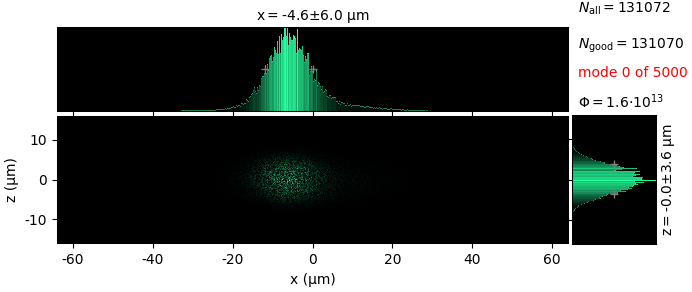
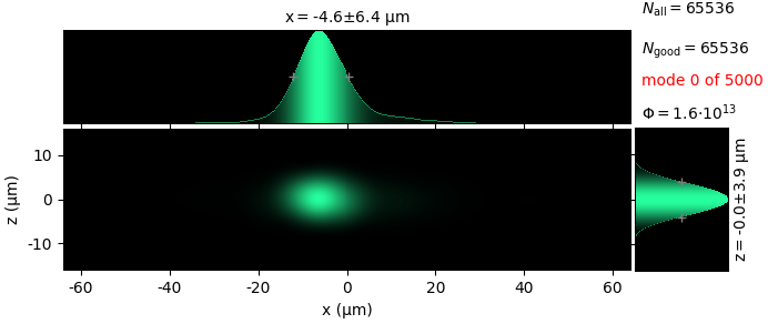
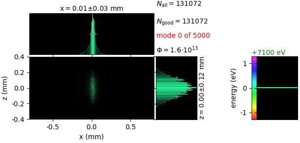
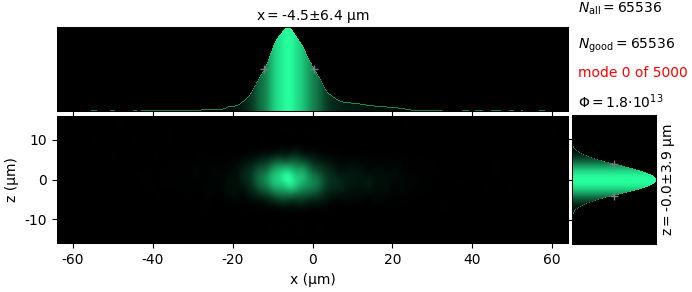
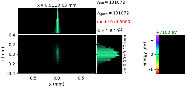
The coherent radiation in the 0th mode has a weight (coherent fraction) ≈3.66%. Here it was individually propagated in three different ways:
focus/source |
FE slit |
|
|---|---|---|
rays |
|
|
hybrid |
|
|
wave |
|
|