Wave propagation (diffraction)

Time dependent diffraction

We start from the Kirchhoff integral theorem in the general (time-dependent) form [Born & Wolf]:

\[V(r,t)=\frac 1{4\pi }\int _S\left\{[V]\frac{\partial }{\partial n} \left(\frac 1 s\right)-\frac 1{\mathit{cs}}\frac{\partial s}{\partial n}\left[\frac{\partial V}{\partial t}\right]-\frac 1 s\left[\frac {\partial V}{\partial n}\right]\right\}\mathit{dS},\]

where the integration is performed over the selected surface \(S\), \(s\) is the distance between the point \(r\) and the running point on surface \(S\), \(\frac{\partial }{\partial n}\) denotes differentiation along the normal on the surface and the square brackets on \(V\) terms denote retarded values, i.e. the values at time \(t − s/c\). \(V\) is a scalar wave here but can represent any component of the actual electromagnetic wave provided that the observation point is much further than the wave length (surface currents are neglected here). \(V\) depends on position and time; this is something what we do not have in ray tracing. We obtain it from ray characteristics by:

\[V(s,t)=\frac 1{\sqrt{2\pi }}\int U_{\omega }(s)e^{-i\omega t}d\omega,\]

where \(U_{\omega }(s)\) is interpreted as a monochromatic wave field and therefore can be associated with a ray. Here, this is any component of the ray polarization vector times its propagation factor \(e^{ikl(s)}\). Substituting it into the Kirchhoff integral yields \(V(r,t)\). As we visualize the wave fields in space and energy, the obtained \(V(r,t)\) must be back-Fourier transformed to the frequency domain represented by a new re-sampled energy grid:

\[U_{\omega '}(r)=\frac 1{\sqrt{2\pi }}\int V(r,t)e^{i\omega 't} \mathit{dt}.\]

Ingredients:

\[ \begin{align}\begin{aligned}[V]\frac{\partial }{\partial n}\left(\frac 1 s\right)=-\frac{(\hat {\vec s}\cdot \vec n)}{s^2}[V],\\\frac 1{\mathit{cs}}\frac{\partial s}{\partial n}\left[\frac{\partial V}{\partial t}\right]=\frac{ik} s(\hat{\vec s}\cdot \vec n)[V],\\\frac 1 s\left[\frac{\partial V}{\partial n}\right]=\frac{ik} s(\hat {\vec l}\cdot \vec n)[V],\end{aligned}\end{align} \]

where the hatted vectors are unit vectors: \(\hat {\vec l}\) for the incoming direction, \(\hat {\vec s}\) for the outgoing direction, both being variable over the diffracting surface. As \(1/s\ll k\), the 1st term is negligible as compared to the second one.

Finally,

\[U_{\omega '}(r)=\frac{-i}{8\pi ^2\hbar ^2c}\int e^{i(\omega '-\omega)t} \mathit{dt}\int \frac E s\left((\hat{\vec s}\cdot \vec n)+(\hat{\vec l} \cdot \vec n)\right)U_{\omega }(s)e^{ik(l(s)+s)}\mathit{dS}\mathit{dE}.\]

The time-dependent diffraction integral is not yet implemented in xrt.

Stationary diffraction

If the time interval \(t\) is infinite, the forward and back Fourier transforms give unity. The Kirchhoff integral theorem is reduced then to its monochromatic form. In this case the energy of the reconstructed wave is the same as that of the incoming one. We can still use the general equation, where we substitute:

\[\delta (\omega -\omega ')=\frac 1{2\pi }\int e^{i(\omega '-\omega )t} \mathit{dt},\]

which yields:

\[U_{\omega }(r)=-\frac {i k}{4\pi }\int \frac1 s\left((\hat{\vec s}\cdot \vec n)+(\hat{\vec l}\cdot \vec n)\right)U_{\omega }(s)e^{ik(l(s)+s)} \mathit{dS}.\]

How we treat non-monochromaticity? We repeat the sequence of ray-tracing from the source down to the diffracting surface for each energy individually. For synchrotron sources, we also assume a single electron trajectory (so called “filament beam”). This single energy contributes fully coherently into the diffraction integral. Different energies contribute incoherently, i.e. we add their intensities, not amplitudes.

The input field amplitudes can, in principle, be taken from ray-tracing, as it was done by [Shi_Reininger] as \(U_\omega(s) = \sqrt{I_{ray}(s)}\). This has, however, a fundamental difficulty. The notion “intensity” in many ray tracing programs, as in Shadow used in [Shi_Reininger], is different from the physical meaning of intensity: “intensity” in Shadow is a placeholder for reflectivity and transmittivity. The real intensity is represented by the density of rays – this is the way the rays were sampled, while each ray has \(I_{ray}(x, z) = 1\) at the source [shadowGuide], regardless of the intensity profile. Therefore the actual intensity must be reconstructed. We tried to overcome this difficulty by computing the density of rays by (a) histogramming and (b) kernel density estimation [KDE]. However, the easiest approach is to sample the source with uniform ray density (and not proportional to intensity) and to assign to each ray its physical wave amplitudes as s and p projections. In this case we do not have to reconstruct the physical intensity. The uniform ray density is an option for the geometric and synchrotron sources in sources.

Notice that this formulation does not require paraxial propagation and thus xrt is more general than other wave propagation codes. For instance, it can work with gratings and FZPs where the deflection angles may become large.

[Shi_Reininger] (1,2)

X. Shi, R. Reininger, M. Sanchez del Rio & L. Assoufid, A hybrid method for X-ray optics simulation: combining geometric ray-tracing and wavefront propagation, J. Synchrotron Rad. 21 (2014) 669–678.

[shadowGuide]

6. Cerrina, “SHADOW User’s Guide” (1998).

[KDE]

Michael G. Lerner (mglerner) (2013) http://www.mglerner.com/blog/?p=28

Normalization

The amplitude factors in the Kirchhoff integral assure that the diffracted wave has correct intensity and flux. This fact appears to be very handy in calculating the efficiency of a grating or an FZP in a particular diffraction order. Without proper amplitude factors one would need to calculate all the significant orders and renormalize their total flux to the incoming one.

The resulting amplitude is correct provided that the amplitudes on the diffracting surface are properly normalized. The latter are normalized as follows. First, the normalization constant \(X\) is found from the flux integral:

\[F = X^2 \int \left(|E_s|^2 + |E_p|^2 \right) (\hat{\vec l}\cdot \vec n) \mathit{dS}\]

by means of its Monte-Carlo representation:

\[X^2 = \frac{F N }{\sum \left(|E_s|^2 + |E_p|^2 \right) (\hat{\vec l}\cdot \vec n) S} \equiv \frac{F N }{\Sigma(J\angle)S}.\]

The area \(S\) can be calculated by the user or it can be calculated automatically by constructing a convex hull over the impact points of the incoming rays. The voids, as in the case of a grating (shadowed areas) or an FZP (the opaque zones) cannot be calculated by the convex hull and such cases must be carefully considered by the user.

With the above normalization factors, the Kirchhoff integral calculated by Monte-Carlo sampling gives the polarization components \(E_s\) and \(E_p\) as (\(\gamma = s, p\)):

\[E_\gamma(r) = \frac{\sum K(r, s) E_\gamma(s) X S}{N} = \sum{K(r, s) E_\gamma(s)} \sqrt{\frac{F S} {\Sigma(J\angle) N}}.\]

Finally, the Kirchhoff intensity \(\left(|E_s|^2 + |E_p|^2\right)(r)\) must be integrated over the screen area to give the flux.

Note

The above normalization steps are automatically done inside diffract().

Sequential propagation

In order to continue the propagation of a diffracted field to the next optical element, not only the field distribution but also local propagation directions are needed, regardless how the radiation is supposed to be propagated further downstream: as rays or as a wave. The directions are given by the gradient applied to the field amplitude. Because \(1/s\ll k\) (validity condition for the Kirchhoff integral), the by far most significant contribution to the gradient is from the exponent function, while the gradient of the pre-exponent factor is neglected. The new wave directions are thus given by a Kirchhoff-like integral:

\[{\vec \nabla } U_{\omega }(r) = \frac {k^2}{4\pi } \int \frac {\hat{\vec s}} s \left((\hat{\vec s}\cdot \vec n)+(\hat{\vec l}\cdot \vec n)\right) U_{\omega }(s)e^{ik(l(s)+s)} \mathit{dS}.\]

The resulted vector is complex valued. Taking the real part is not always correct as the vector components may happen to be (almost) purely imaginary. Our solution is to multiply the vector components by a conjugate phase factor of the largest vector component and only then to take the real part.

The correctness of this approach to calculating the local wave directions can be verified as follows. We first calculate the field distribution on a flat screen, together with the local directions. The wave front, as the surface normal to these directions, is calculated by linear integrals of the corresponding angular projections. The calculated wave front surface is then used as a new screen, where the diffracted wave is supposed to have a constant phase. This is indeed demonstrated in the example applying phase as color axis. The sharp phase distribution is indicative of a true wave front, which in turn justifies the correct local propagation directions.

After having found two polarization components and new directions on the receiving surface, the last step is to reflect or refract the wave samples as rays locally, taking the complex refractive indices for both polarizations. This approach is applicable also to wave propagation regime, as the reflectivity values are purely local to the impact points.

Usage

Warning

You need a good graphics card for running these calculations!

Note

OpenCL platforms/devices can be inspected in xrtQook (‘GPU’ button)

Warning

Long calculation on GPU in Windows may result in the system message “Display driver stopped responding and has recovered” or python RuntimeError: out of resources (yes, it’s about the driver response, not the lack of memory). The solution is to change TdrDelay registry key from the default value of 2 seconds to some hundreds or even thousands. Please refer to https://msdn.microsoft.com/en-us/library/windows/hardware/ff569918(v=vs.85).aspx

Tip

If you plan to utilize xrt on a multi-GPU platform under Linux, we recommend KDE based systems (e.g. Kubuntu). It is enough to install the package fglrx-updates-dev without the complete graphics driver.

In contrast to ray propagation, where passing through an optical element requires only one method (“reflect” for a reflective/refractive surface or “propagate” for a slit), wave propagation in our implementation requires two or three methods:

1. prepare_wave creates points on the receiving surface where the diffraction integral will be calculated. For an optical element or a slit the points are uniformly randomly distributed (therefore reasonable physical limits must be given); for a screen the points are determined by the screen pixels. The returned wave is an instance of class Beam, where the arrays x, y, z are local to the receiving surface.

2. diffract (as imported function from xrt.backends.raycing.waves or as a method of the diffracted beam) takes a beam local to the diffracting surface and calculates the diffraction integrals at the points prepared by prepare_wave. There are five scalar integrals: two for Es and Ep and three for the components of the diffracted direction (see the previous Section). All five integrals are calculated in the coordinates local to the diffracting surface but at the method’s end these are transformed to the local coordinates of the receiving surface (remained in the wave container) and to the global coordinate system (a Beam object returned by diffract).

For slits and screens, the two steps above are sufficient. For an optical element, another step is necessary.

3. reflect method of the optical element is meant to take into account its material properties. The intersection points are already known (unless the optical element is distorted, i.e. has methods local_z_distorted and local_n_distorted), as provided by the previous prepare_wave. This fact (knowledge of the intersection points) can be reported to reflect by noIntersectionSearch=True. Here, reflect takes the beam right before the surface and propagates it to right after it. As a result of such a zero-length travel, the wave gets no additional propagation phase but only a complex-valued reflectivity coefficient and a new propagation direction. Note that for parametric or distorted OEs this last-stroke travel is not zero-length but the propagation phase is properly taken into account.

These three methods are enough to describe wave propagation through the complete beamline. The first two methods, prepare_wave and diffract, are split from each other because the diffraction calculations may need several repeats in order to accumulate enough wave samples for attaining dark field at the image periphery. The second method can reside in a loop that will accumulate the complex valued field amplitudes in the same beam arrays defined by the first method. In the supplied examples, prepare_wave for the last screen is done before a loop and all the intermediate diffraction steps are done within that loop.

The quality of the resulting diffraction images is mainly characterized by the blackness of the dark field – the area of expected zero intensity. If the statistics is not sufficient, the dark area is not black, and can even be bright enough to mask the main spot. The contrast depends both on beamline geometry (distances) and on the number of wave field samples (a parameter for prepare_wave). Shorter distances require more samples for the same quality, and for the distances shorter than a few meters one may have to reduce the problem dimensionality by cutting in horizontal or vertical, see the examples of SoftiMAX. In the console output, diffract reports on samples per zone (meaning per Fresnel zone). As a rule of thumb, this figure should be greater than ~10⁴ for a good resulting quality.

OE.prepare_wave(prevOE, nrays, shape='auto', area='auto', rw=None)

Creates the beam arrays used in wave diffraction calculations. prevOE is the diffracting element: a descendant from OE, RectangularAperture or RoundAperture. nrays: if int, specifies the number of randomly distributed samples the surface within self.limPhysX limits; if 2-tuple of ints, specifies (nx, ny) sizes of a uniform mesh of samples; if 2-tuple of arrays, specifies the (x, y) positions.

RectangularAperture.prepare_wave(prevOE, nrays, rw=None)

Creates the beam arrays used in wave diffraction calculations. prevOE is the diffracting element: a descendant from OE, RectangularAperture or RoundAperture. nrays of samples are randomly distributed over the slit area.

Screen.prepare_wave(prevOE, dim1, dim2, dy=0, rw=None, condition=None)

Creates the beam arrays used in wave diffraction calculations. prevOE is the diffracting element: a descendant from OE, RectangularAperture or RoundAperture. dim1 and dim2 are x and z arrays for a flat screen or phi and theta arrays for a hemispheric screen. The two arrays are generally of different 1D shapes. They are used to create a 2D mesh by meshgrid.

condition: a callable defined in the user script with two flattened

meshgrid arrays as inputs and outputs. Can be used to select wave samples. An example:

def condition(d1s, d2s):
    cond = d1s**2 + d2s**2 <= pinholeDia**2 / 4  # in a pinhole
    return d1s[cond], d2s[cond]

xrt.backends.raycing.waves.diffract(oeLocal, wave, targetOpenCL='auto', precisionOpenCL='auto')

Calculates the diffracted field – the amplitudes and the local directions – contained in the wave object. The field on the diffracting surface is given by oeLocal. You can explicitly change OpenCL settings targetOpenCL and precisionOpenCL which are initially set to ‘auto’, see their explanation in xrt.backends.raycing.sources.Undulator.

Coherence signatures

A standard way to define coherence properties is via mutual intensity J (another common name is cross-spectral density) and complex degree of coherence j (DoC, normalized J):

\[\begin{split}J(x_1, y_1, x_2, y_2) \equiv J_{12} = \left<E(x_1, y_1)E^{*}(x_2, y_2)\right>\\ j(x_1, y_1, x_2, y_2) \equiv j_{12} = \frac{J_{12}}{\left(J_{11}J_{22}\right)^{1/2}},\end{split}\]

where the averaging \(\left<\ \right>\) in \(J_{12}\) is over different realizations of filament electron beam (one realization per repeat) and is done for the field components \(E_s\) or \(E_p\) of a field diffracted onto a given \((x, y)\) plane.

Both functions are Hermitian in respect to the exchange of points 1 and 2. There are two common ways of working with them:

1. The horizontal and vertical directions are considered independently by placing the points 1 and 2 on a horizontal or vertical line symmetrically about the optical axis. DoC thus becomes a 1D function dependent on the distance between the points, e.g. as \(j_{12}^{\rm hor}=j(x_1-x_2)\). The intensity distribution is also determined over the same line as a 1D positional function, e.g. as \(I(x)\).

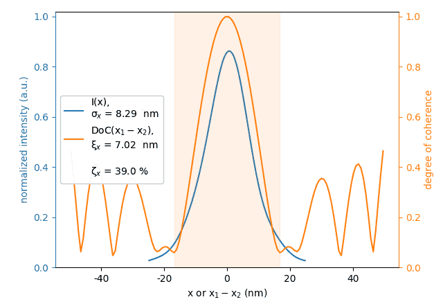
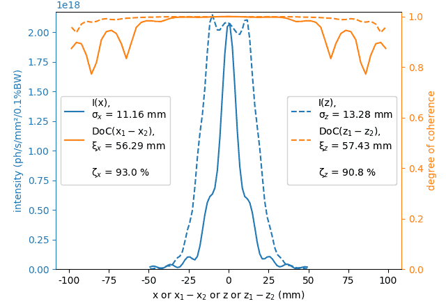
   The widths \(\sigma_x\) and \(\xi_x\) of the distributions \(I(x)\) and \(j(x_1-x_2)\) give the coherent fraction \(\zeta_x\) [Vartanyants2010]

   \[\zeta_x = \left(4\sigma_x^2/\xi_x^2 + 1\right)^{-1/2}.\]

2. The transverse field distribution can be analized integrally (not split into the horizontal and vertical projections) by performing the modal analysis consisting of solving the eigenvalue problem for the matrix \(J^{tr=1}_{12}\) – the matrix \(J_{12}\) normalized to its trace – and doing the standard eigendecomposition:

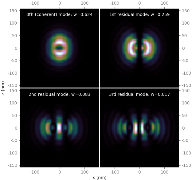
   \[J^{tr=1}(x_1, y_1, x_2, y_2) = \sum_i{w_i V_i(x_1, y_1)V_i^{+}(x_2, y_2)},\]

   with \(w_i, V_i\) being the ith eigenvalue and eigenvector. \(w_0\) is the fraction of the total flux contained in the 0th (coherent) mode or coherent flux fraction.

   Note

   The matrix \(J_{12}\) is of the size (N_x×N_y)², i.e. squared total pixel size of the image! In the current implementation, we use eigh() method from scipy.linalg, where a feasible image size should not exceed ~100×100 pixels (i.e. ~10⁸ size of \(J_{12}\)).

   Note

   For a fully coherent field \(j_{12}\equiv1\) and \(w_0=1, w_i=0\ \forall i>0\), \(V_0\) being the coherent field.

We also propose a third method that results in the same figures as the second method above.

3. It uses Principal Component Analysis (PCA) applied to the filament images \(E(x, y)\). It consists of the following steps.

   1. Out of r repeats of \(E(x, y)\) build a stacked data matrix \(D\) with N_x×N_y rows and r columns.

   2. The matrix \(J_{12}\) is equal to the product \(DD^{+}\). Instead of solving this huge eigenvalue problem of (N_x×N_y)² size, we solve a typically smaller covariance matrix \(D^{+}D\) of the size r².

   3. The spectra of eigenvalues of matrices \(DD^{+}\) and \(D^{+}D\) are equal, plus zeroes for the bigger matrix.

   4. Their eigenvectors (being eigenmodes \(V_i\) of \(DD^{+}\) and principal component axes \(v_i\) of \(D^{+}D\)) corresponding to the same eigenvalue are transformed to each other with a factor \(D\) or \(D^{+}\): \(\tilde{V}_i = Dv_i\) and \(\tilde{v}_i = D^{+}V_i\), after which transformation they must be additionally normalized (\(\tilde{v}_i\) and \(\tilde{V}_i\) are non-normalized eigenvectors) [the proof is a one line matrix equation].

   Finally, PCA gives exactly the same information as the direct modal analysis (method No 2 above) but is cheaper to calculate by many orders of magnitude.

One can define another measure of coherence as a single number, termed as degree of transverse coherence (DoTC) [Saldin2008]:

\[{\rm DoTC} = \frac{\iiiint |J_{12}|^2 dx_1 dy_1 dx_2 dy_2} {\left[\iint J_{11} dx_1 dy_1\right]^2}\]

[Saldin2008]

E.L. Saldin, E.A. Schneidmiller, M.V. Yurkov, Coherence properties of the radiation from X-ray free electron laser, Opt. Commun. 281 (2008) 1179–88.

[Vartanyants2010]

I.A. Vartanyants and A. Singer, Coherence properties of hard x-ray synchrotron sources and x-ray free-electron lasers, New Journal of Physics 12 (2010) 035004.

We propose to calculate DoTC from the matrix traces [derivation to present in the coming paper] as:

4. 1. DoTC = Tr(J²)/Tr²(J).

   2. DoTC = Tr(D⁺DD⁺D)/Tr²(D⁺D), with the matrix D defined above. The exactly same result as in (a) but obtained with smaller matrices.

Note

A good test for the correctness of the obtained coherent fraction is to find it at various positions on propagating in free space, where the result is expected to be invariant. As appears in the examples of SoftiMAX, the analysis based on DoC never gives an invariant coherent fraction at the scanned positions around the focus. The primary reason for this is the difficulty in the determination of the width of DoC, for the latter typically being a complex-shaped oscillatory curve. In contrast, the modal analysis (the PCA implementation is recommended) and the DoTC give the expected invariance.

Coherence analysis and related plotting

The module coherence has functions for 1D and 2D analysis of coherence and functions for 1D plotting of degree of coherence and and 2D plotting of eigen modes.

The input for the analysis functions is a 3D stack of field images. It can be obtained directly from the undulator class, or from a plot object after several repeats of wave propagation of a filament beam through a beamline. Examples can be found in ...\tests\raycing\test_coherent_fraction_stack.py and in SoftiMAX at MAX IV.

xrt.backends.raycing.coherence.calc_1D_coherent_fraction(U, axisName, axis, p=0)

Calculates 1D degree of coherence (DoC). From its width in respect to the width of intensity distribution also infers the coherent fraction. Both widths are rms. The one of intensity is calculated over the whole axis, the one of DoC is calculated between the first local minima around the center provided that these minima are lower than 0.5.

U: complex valued ndarray, shape(repeats, nx, ny)

3D stack of field images. For a 1D cut along axis, the middle of the other dimension is sliced out.

axis: str, one of ‘x’ or (‘y’ or ‘z’)

Specifies the 1D axis of interest.

p: float, distance to screen

If non-zero, the calculated mutual intensity will be divided by p². This is useful to get proper physical units of the returned intensity if the function is applied directly to the field stacks given by Undulator.multi_electron_stack() that is calculated in angular units.

Returns a tuple of mutual intensity, 1D intensity, 1D DoC, rms width of intensity, rms width of DoC (between the local minima, see above), the position of the minima (only the positive side) and the coherent fraction. This tuple can be fed to the plotting function plot_1D_degree_of_coherence().

xrt.backends.raycing.coherence.plot_1D_degree_of_coherence(data1D, axisName, axis, unit='mm', fig2=None, isIntensityNormalized=False, locLegend='auto')

Provides two plots: a 2D plot of mutual intensity and a 1D plot of intensity and DoC. The latter plot can be shared between the two 1D axes if this function is invoked two times.

data1D: tuple returned by calc_1D_coherent_fraction().

axisName: str, used in labels.

axis: 1D array of abscissa.

unit: str, used in labels.

fig2: matplotlib figure object, if needed for shared plotting of two 1D axes.

isIntensityNormalized: bool, controls the intensity axis label.

locLegend: str, legend location in matplotlib style.

Returns the two figure objects for the user to add suptitles and to export to image files.

Plot examples for one and two 1D curves:

xrt.backends.raycing.coherence.calc_degree_of_transverse_coherence_4D(J)

Calculates DoTC from the mutual intensity J as Tr(J²)/Tr²(J). This function should only be used for demonstration purpose. There is a faster alternative: calc_degree_of_transverse_coherence_PCA().

xrt.backends.raycing.coherence.calc_degree_of_transverse_coherence_PCA(U)

Calculates DoTC from the field stack U. The field images of U are flattened to form the matrix D shaped as (repeats, nx×ny). DoTC = Tr(D⁺DD⁺D)/Tr²(D⁺D), which is equal to the original DoTC for the mutual intensity J: DoTC = Tr(J²)/Tr²(J).

xrt.backends.raycing.coherence.calc_eigen_modes_4D(J, eigenN=4)

Solves the eigenvalue problem for the mutual intensity J. This function should only be used for demonstration purpose. There is a much faster alternative: calc_eigen_modes_PCA().

xrt.backends.raycing.coherence.calc_eigen_modes_PCA(U, eigenN=4, maxRepeats=None, normalize=False)

Solves the PCA problem for the field stack U shaped as (repeats, nx, ny). The field images are flattened to form the matrix D shaped as (repeats, nx×ny). The eigenvalue problem is solved for the matrix D⁺*D*.

Returns a tuple of two arrays: eigenvalues in a 1D array and eigenvectors as columns of a 2D array. This is a much faster and exact replacement of the full eigen mode decomposition by calc_eigen_modes_4D().

eigenN sets the number of returned eigen modes. If None, the number of modes is inferred from the shape of the field stack U and is equal to the number of macroelectrons (repeats). If given as a 2-tuple, eigenN refers to the number of eigenvalues and eigenvectors separately.

if maxRepeats are given, the stack is sliced up to that number. This option is introduced in order not to make the eigenvalue problem too big.

If normalize is True, the eigenvectors are normalized, otherwise they are the PCs of the field stack in the original field units.

xrt.backends.raycing.coherence.plot_eigen_modes(x, y, w, v, xlabel='', ylabel='', aspect=1)

Provides 2D plots of the first 4 eigen modes in the given x and y coordinates. The eigen modes are specified by eigenvalues and eigenvectors w and v returned by calc_eigen_modes_PCA() or calc_eigen_modes_4D().

Plot example:

Typical logic for a wave propagation study

1. According to [Wolf], the visibility is not affected by a small bandwidth. It is therefore recommended to first work with strictly monochromatic radiation and check non-monochromaticity at the end.

2. Do a hybrid propagation (waves start somewhere closer to the end) at zero emittance. Put the screen at various positions around the main focus for seeing the depth of focus.

3. Examine the focus and the footprints and decide if vertical and horizontal cuts are necessary (when the dark field does not become black enough at a reasonably high number of wave samples).

4. Run non-zero electron emittance, which spoils both the focal size and the degree of coherence.

5. Try various ways to improve the focus and the degree of coherence: e.g. decrease the exit slit or elongate inter-optics distances.

6. Do hybrid propagation for a finite energy band to study the chromaticity in focus position.

[Wolf]

E. Wolf. Introduction to the theory of coherence and polarization of light. Cambridge University Press, Cambridge, 2007.