Sources

Beam	Container for beam arrays and variables, see listOfAttrs.
GeometricSource	Geometric source - a source with the ray origin, divergence and energy sampled with given distribution laws.
MeshSource	Point source of a rectangular angular mesh of divergent rays.
CollimatedMeshSource	Mesh of collimated rays, similarly to MeshSource.
GaussianBeam	Gaussian beam https://en.wikipedia.org/wiki/Gaussian_beam.
LaguerreGaussianBeam	Laguerre-Gaussian version of GaussianBeam.
HermiteGaussianBeam	Hermite-Gaussian version of GaussianBeam.
BendingMagnetWS	Bending magnet source that uses the external code ws (legacy source).
WigglerWS	Wiggler source that uses the external code ws (legacy source).
UndulatorUrgent	Undulator source that uses the external code urgent (legacy source).
SourceBase	Base class for all internal synchrotron sources of xrt, not to be called explicitly.
BendingMagnet	Bending magnet source based on a simplified analytical radiation model for a constant magnetic field.
Wiggler	Wiggler source modeled as an incoherent sum of bending magnet sources.
IntegratedSource	Base class for xrt sources with numerically integrated amplitudes: Undulator and SourceFromField.
Undulator	Undulator source that calculates electric field amplitudes by numerical integration along the electron trajectory in a sinusoidal magnetic field, including fields with varying amplitude (tapered undulators).
SourceFromField	Synchrotron source that calculates electric-field amplitudes through numerical integration along the electron trajectory in a user-defined 3D magnetic field․ It accepts tabulated magnetic fields derived from analytical models or measurements and supports quasi-periodic undulators, custom-field wigglers, bending-magnet edge radiation, and virtually any magnetic-field configuration.

Sampling strategies

There are three main strategies for creating samples of optical sources, depending on study purpose, implemented in xrt.

1. Monte Carlo sampling by intensity, or ray generation. This is the default mode of all synchrotron sources in xrt and is the best sampling strategy for ray tracing or hybrid wave propagation (when the wave part starts at a downstream optical element). Technically it is done by the acceptance-rejection method. In this method, the optical field is calculated in a 3D space – energy and two transverse angles – for a set of uniformly random values of these three variables within the predefined ranges. The transverse angles also get normally distributed angular shifts within the emittance distribution, independently for each ray. The acceptance random variable is uniformly sampled in the range from zero to the intensity maximum for each field sample, and the sample is accepted if the acceptance variable is below the sample intensity, otherwise it is rejected. The sampling continues until the requested number of samples is reached. The resulted space density of the samples (rays) is proportional to the field intensity.

2. Uniform Monte Carlo sampling, or wave generation. This mode is necessary for wave propagation when it starts right from the source. The 3D calculation space – energy and two transverse angles – is sampled uniformly. This way of sampling is still possible to use for ray tracing, and it is even faster at the source as no samples are rejected, but it is less efficient at the downstream part of the beamline as a significant part of the samples (or even a majority of them) is of low intensity. The main usage pattern of this sampling is, however, for single electron (or macro electrons) field propagation (enabled by the source option filamentBeam=True), when all wave samples are attributed to the same electron with a single displacement within emittance distribution and a single shift of gamma (relative electron energy) within energy spread distribution.

3. Grid sampling. This is frequently a quick method for studying synchrotron sources in reciprocal space and energy that must be used with care as it is full of pitfalls. Grid samples can be obtained by intensities_on_mesh() method of the synchrotron source. Three aspects must be considered when making a grid. (i) For a sharp field distribution, e.g. for an undulator at zero emittance and zero electron beam energy spread, the sharp field rings may interfere with the grid (form moiré patterns) and result in false fringes in spectral flux density. In such cases, the grid has to be very finely spaced. (ii) When the electron beam emittance is non-zero, the calculated field values have to be convolved with the electron beam divergence; this convolution is done inside intensities_on_mesh(). Due to the edge effects of the convolution, the grid borders of the thickness of the doubled electron beam divergence must be discarded from the field arrays returned by intensities_on_mesh() and therefore these grid margins have to be added beforehand. (iii) The number of energy spread samples must be set sufficient for the used energy spread value, see the end of the next paragraph.

Electron beam energy spread is treated differently in the above three sampling strategies. In ray sampling, every ray gets its gamma sample (relative electron energy) of the normal energy spread distribution. In wave sampling, energy spread is sampled once for all wave samples when in filamentBeam regime and individually per wave sample otherwise. In grid sampling, a new grid dimension is introduced internally that contains samples of gamma within energy spread distribution with subsequent averaging over that dimension. Notice that a wide energy spread distribution (that can be a case for linacs) may require more energy spread samples (the parameter eSpreadNSamples of intensities_on_mesh()) than the default number 36 that is usually good for energy spread sigma of 0.1%. Because of this new dimension, the grid may become too large to fit into RAM, which might force the user to invoke the method intensities_on_mesh() in a loop that scans over individual photon energies.

Electron beam real space size is also treated differently in the above three sampling strategies. In ray sampling, every ray gets its transverse origin shift in the source plane within emittance distribution. In wave sampling, the wave source position is sampled once for all wave samples when in filamentBeam regime and individually per wave sample otherwise. In grid sampling, real space electron beam size is totally ignored.

See the example Undulator radiation through rectangular aperture, where several calculation methods are compared.

Absolute flux and power

Raycing plots calculate flux and power from the ray intensities already carried by the beam. For total flux, the per-ray intensity is the trace of the coherency matrix,

\[I_i = J_{ss,i} + J_{pp,i}.\]

For power plots, the same ray intensity is multiplied by photon energy and by the joule-per-eV conversion factor,

\[P_i = I_i E_i e,\]

where \(E_i\) is in eV.

If a beam has sourceWeight, raycing treats it as the source normalization represented by the ray. For a run with \(N\) rays, the histogram receives

\[N I_i w_i\]

for flux, or

\[N I_i E_i e w_i\]

for power, where \(w_i\) is beam.sourceWeight. The reported plot value is divided by the accumulated number of rays, so for one run this is equivalent to

\[\Phi = \sum_i I_i w_i,\]

and

\[P = \sum_i I_i E_i e w_i.\]

The same logic applies to the selected subset of rays in a plot, and to the other fluxKind values with the corresponding coherency-matrix component in place of \(J_{ss}+J_{pp}\).

For synchrotron sources, sourceWeight is determined by the sampled source bounding volume. In the usual far-field ray source this volume is

\[V = (E_{\max} - E_{\min}) (\Theta_{\max} - \Theta_{\min}) (\Psi_{\max} - \Psi_{\min}).\]

The calculated source intensity at a sampled point is denoted below as \(F_i\).

With rejection sampling, trial points are sampled uniformly in this volume. Only a subset is accepted, and the accepted rays have unit initial total intensity. If \(M\) trial points were tested, raycing estimates the source normalization as

\[C = {V \over M}\sum_{k=1}^{M} F_k.\]

If \(N\) rays are accepted and propagated, each propagated ray gets

\[w_i = {C \over N}.\]

Then, for any downstream transmission or selection factor \(T_i\),

\[\Phi = \sum_i T_i w_i = {C \over N}\sum_i T_i \rightarrow \int_V T(\xi) F(\xi)\,d\xi.\]

With uniform ray density, all sampled points are used and the calculated source intensity is carried by the ray intensities themselves. Raycing stores

\[w_i = \frac{V}{N}.\]

The plot flux is then

\[\Phi = \sum_i T_i F_i {V \over N} \rightarrow \int_V T(\xi) F(\xi)\,d\xi.\]

Thus both sampling modes use the same plot-side calculation; they differ only in where the source intensity is represented: in ray density for rejection sampling, or in ray weights for uniform ray density. Power is calculated by the same estimator with the additional factor \(E_i e\).

For geometric sources, there is no calculated synchrotron intensity map. If totalFlux is supplied, raycing normalizes the generated beam directly. Let

\[I_i^0 = J_{ss,i}^0 + J_{pp,i}^0\]

be the initial ray intensity after polarization and any source-specific amplitude weighting. Raycing sets

\[w_i = \frac{\Phi_0}{\sum_j I_j^0},\]

where \(\Phi_0\) is totalFlux. Therefore the source beam satisfies

\[\sum_i I_i^0 w_i = \Phi_0.\]

After propagation, the plotted flux is the same weighted sum of the remaining ray intensities,

\[\Phi = \sum_i I_i w_i,\]

and power is

\[P = \sum_i I_i E_i e w_i.\]

This also works for geometric sources generated with uniform ray density, because the normalization uses the actual initial ray intensities.

The normalization is local to each ray, so it survives beam concatenation. If two beams are concatenated, their ray arrays and their sourceWeight values are concatenated together. The combined plot value is therefore

\[\Phi_{A+B} = \sum_{i \in A} I_i w_i + \sum_{j \in B} I_j w_j = \Phi_A + \Phi_B,\]

and likewise for power. This is useful, for example, for adding independent sources such as canted or serial insertion devices, or an insertion device and a bending magnet. The addition is an incoherent sum of ray intensities.

Grid sampling does not use these beam counters. Its absolute flux and power are obtained by directly integrating the intensity map, or the intensity map multiplied by photon energy, over the grid.

Beam container

Beam.listOfAttrs = ['x', 'y', 'z', 'sourceSIGMAx', 'sourceSIGMAz', 'filamentDX', 'filamentDZ', 'filamentDtheta', 'filamentDpsi', 'filamentDgamma', 'state', 'a', 'b', 'c', 'path', 'E', 'Jss', 'Jpp', 'Jsp', 'elevationD', 'elevationX', 'elevationY', 'elevationZ', 's', 'phi', 'r', 'theta', 'order', 'accepted', 'acceptedE', 'seeded', 'seededI', 'Es', 'Ep', 'nRefl', 'sourceWeight']

class xrt.backends.raycing.sources.Beam(nrays=100000, copyFrom=None, forceState=False, withNumberOfReflections=False, withAmplitudes=False, xyzOnly=False, bl=None)

Container for beam arrays and variables, see listOfAttrs.

x, y, z: float

Starting points of the rays.

a, b, c: float

Normalized vectors of ray directions (the source is responsible for the normalization).

E: float

Energy.

state: int

Per-ray propagation state. See Beam categories.

Jss, Jpp, Jsp: float, float, complex

Components of the coherency matrix.

Es, Ep: complex

S- and p-polarized field amplitudes (not always used).

path: float

Total path length from the source to the last impact point.

theta: float

Incidence angle.

order: int

Order of grating diffraction.

If multiple reflections are considered:

nRefl: int

Number of reflections,

elevationD: float

Maximum elevation distance between the rays and the surface as the ray travels from one impact point to the next one,

elevationX, elevationY, elevationZ: float

Coordinates of the highest elevation points.

If an OE uses a parametric representation:

s, phi, r: float

Arrays storing the impact points in the parametric coordinates.

concatenate(beam)

Adds beam to self. Useful when more than one source is presented.

export_beam(fileName, fformat='npy')

Saves the beam to a binary file. File format can be Numpy ‘npy’, Matlab ‘mat’ or python ‘pickle’. Matlab format should not be used for future imports in xrt as it does not allow correct load.

Geometric sources

Module sources defines the container class Beam that holds beam properties as numpy arrays and defines the beam sources. The sources are geometric sources in continuous and mesh forms and synchrotron sources.

The intensity and polarization of each ray are determined via coherency matrix. This way is appropriate for incoherent addition of rays, in which the components of the coherency matrix of different rays are simply added.

class xrt.backends.raycing.sources.GeometricSource

Geometric source - a source with the ray origin, divergence and energy sampled with given distribution laws.

__init__(bl=None, name='', center=(0, 0, 0), nrays=100000, distx='normal', dx=0.32, disty=None, dy=0, distz='normal', dz=0.018, distxprime='normal', dxprime=0.001, distzprime='normal', dzprime=0.0001, distE='lines', energies=(9000.0,), energyWeights=None, polarization='horizontal', filamentBeam=False, uniformRayDensity=False, pitch=0, roll=0, yaw=0, totalFlux=None, **kwargs)

bl: instance of BeamLine

name: str

center: tuple of 3 floats

3D point in global system

nrays: int

distx, disty, distz, distxprime, distzprime:

Linear (distx, disty, distz) and angular (distxprime, distzprime) source distributions. Accepted values: ‘normal’, ‘flat’, ‘annulus’ or None. If is None, the corresponding arrays remain with the values got at the instantiation of Beam. ‘annulus’ sets a uniform distribution for (x and z) or for (xprime and zprime) pairs. You can assign ‘annulus’ to only one member in the pair.

dx, dy, dz, dxprime, dzprime: float

Linear (dx, dy, dz) and angular (dxprime, dzprime) source sizes. For normal distribution is sigma or (sigma, cut_limit), for flat is full width or tuple (min, max), for annulus is tuple (rMin, rMax), otherwise is ignored.

distE: ‘normal’, ‘flat’, ‘lines’, None

energies: all in eV. (centerE, sigmaE) for distE = ‘normal’,

(minE, maxE) for distE = ‘flat’, a sequence of E values for distE = ‘lines’

Note

Erroneous input (size/type mismatch) will default to monochromatic distribution. If sigmaE exceeds 10% of centerE, sigmaE is taken as zero to avoid sampling negative energies.

energyWeights: 1-D array-like

Can be used together with distE = ‘lines’ to specify the weight of each line. Must be of the shape of energies.

polarization:

‘h[orizontal]’, ‘v[ertical]’, ‘+45’, ‘-45’, ‘r[ight]’, ‘l[eft]’, None, numeric angle in degrees, custom. In the latter case the polarization is given by a sequence of 4 components of the coherency matrix: (Jss, Jpp, Re(Jsp), Im(Jsp)).

filamentBeam: bool

If True the source generates coherent monochromatic wavefronts. Required for the wave propagation calculations.

uniformRayDensity: bool

If True, the radiation is sampled uniformly but with varying amplitudes, otherwise with the density proportional to intensity and with constant amplitudes. Required as True for wave propagation calculations. False is usual for ray-tracing. This parameter only affects normal distributions, as for flat and annulus distributions the density is already uniform. If you set it True, the size parameter (dx or dz) will use a +/-5 sigma sampling interval. Use (sigma, cut_limit) sequence to set this half-width explicitly.

See Absolute flux and power for how ray density and ray weights affect plot intensity and normalization.

pitch, roll, yaw: float

rotation angles around x, y and z axes. Useful for canted sources.

totalFlux: float or None

Absolute source flux in ph/s to use for source normalization. The normalization is preserved during propagation and beam concatenation. If None, plot values remain relative intensities or weighted ray counts.

class xrt.backends.raycing.sources.MeshSource

Point source of a rectangular angular mesh of divergent rays. Primarily, it is meant for internal usage for matching the maximum divergence to the optical sizes of optical elements.

__init__(bl=None, name='', center=(0, 0, 0), minxprime=-0.0001, maxxprime=0.0001, minzprime=-0.0001, maxzprime=0.0001, nx=11, nz=11, distE='lines', energies=(9000.0,), energyWeights=None, polarization='horizontal', withCentralRay=True, autoAppendToBL=False, totalFlux=None, **kwargs)

bl: instance of BeamLine

name: str

center: tuple of 3 floats

3D point in global system

minxprime, maxxprime, minzprime, maxzprime: float

limits for the ungular distributions

nx, nz: int

numbers of points in x and z dircetions

distE: ‘normal’, ‘flat’, ‘lines’, None

energies, all in eV: (centerE, sigmaE) for distE = ‘normal’,

(minE, maxE) for distE = ‘flat’, a sequence of E values for distE = ‘lines’

Note

Erroneous input (size/type mismatch) will default to monochromatic distribution. If sigmaE exceeds 10% of centerE, sigmaE is taken as zero to avoid sampling negative energies.

energyWeights: 1-D array-like

Can be used together with distE = ‘lines’ to specify the weight of each line. Must be of the shape of energies.

polarization: ‘h[orizontal]’, ‘v[ertical]’, ‘+45’, ‘-45’, ‘r[ight]’,

‘l[eft]’, None, numeric angle in degrees, custom. In the latter case the polarization is given by a sequence of 4 components of the coherency matrix: (Jss, Jpp, Re(Jsp), Im(Jsp)).

withCentralRay: bool

if True, the 1st ray in the beam is along the nominal beamline direction

autoAppendToBL: bool

if True, the source is added to the list of beamline sources. Otherwise the user must manually start it with shine().

totalFlux: float or None

Absolute source flux in ph/s to use for source normalization. The normalization is preserved during propagation and beam concatenation. If None, plot values remain relative intensities or weighted ray counts.

class xrt.backends.raycing.sources.CollimatedMeshSource(bl=None, name='', center=(0, 0, 0), dx=1.0, dz=1.0, nx=11, nz=11, distE='lines', energies=(9000.0,), energyWeights=None, polarization='horizontal', withCentralRay=True, autoAppendToBL=False, totalFlux=None, **kwargs)

Mesh of collimated rays, similarly to MeshSource.

class xrt.backends.raycing.sources.GaussianBeam(*args, **kwargs)

Gaussian beam https://en.wikipedia.org/wiki/Gaussian_beam.

Warning

Without a prepared wave it generates geometric rays, which is primarily meant for visualization.

With a wave obtained by prepare_wave() of a slit, oe or screen, it calculates the Gaussian field at the available 3D points. See an example in tests/raycing/laguerre_hermite_gaussian_beam.py.

__init__(*args, **kwargs)

w0: float or 2-sequence

Gaussian beam waist size. If a 2-sequence, the sizes refer to the horizontal and the vertical axes.

nrays: int

Number of rays generated when no wave is supplied to shine().

class xrt.backends.raycing.sources.LaguerreGaussianBeam(*args, **kwargs)

Laguerre-Gaussian version of GaussianBeam. It must be used for an already available set of 3D points which are obtained by prepare_wave() of a slit, oe or screen. See a usage example in tests/raycing/laguerre_hermite_gaussian_beam.py.

__init__(*args, **kwargs)

vortex: None or tuple(l, p)

specifies Laguerre-Gaussian beam with l the azimuthal index and p >= 0 the radial index.

class xrt.backends.raycing.sources.HermiteGaussianBeam(*args, **kwargs)

Hermite-Gaussian version of GaussianBeam. It must be used for an already available set of 3D points which are obtained by prepare_wave() of a slit, oe or screen. See a usage example in tests/raycing/laguerre_hermite_gaussian_beam.py.

__init__(*args, **kwargs)

TEM: None or tuple(m, n)

specifies Hermite-Gaussian beam of order (m, n) referring to the x and y directions.

xrt.backends.raycing.sources.make_energy(distE, energies, nrays, filamentBeam=False, energyWeights=None)

Creates energy distributions with the distribution law given by distE. energies either determine the limits or is a sequence of discrete energies. If distE is ‘lines’, energyWeights can define the relative weights of the lines.

xrt.backends.raycing.sources.make_polarization(polarization, bo, nrays=100000)

Initializes the coherency matrix. The following polarizations are supported:

1. horizontal (polarization is a string started with ‘h’):

   \[\begin{split}J = \left( \begin{array}{ccc}1 & 0 \\ 0 & 0\end{array} \right)\end{split}\]

2. vertical (polarization is a string started with ‘v’):

   \[\begin{split}J = \left( \begin{array}{ccc}0 & 0 \\ 0 & 1\end{array} \right)\end{split}\]

3. at +45º (polarization = ‘+45’):

   \[\begin{split}J = \frac{1}{2} \left( \begin{array}{ccc}1 & 1 \\ 1 & 1\end{array} \right)\end{split}\]

4. at -45º (polarization = ‘-45’):

   \[\begin{split}J = \frac{1}{2} \left( \begin{array}{ccc}1 & -1 \\ -1 & 1\end{array} \right)\end{split}\]

5. right (polarization is a string started with ‘r’):

\[\begin{split}J = \frac{1}{2} \left( \begin{array}{ccc}1 & i \\ -i & 1\end{array} \right)\end{split}\]

5. left (polarization is a string started with ‘l’):

   \[\begin{split}J = \frac{1}{2} \left( \begin{array}{ccc}1 & -i \\ i & 1\end{array} \right)\end{split}\]

7. unpolarized (polarization is None):

   \[\begin{split}J = \frac{1}{2} \left( \begin{array}{ccc}1 & 0 \\ 0 & 1\end{array} \right)\end{split}\]

8. user-defined (polarization is 4-sequence with):

   \[\begin{split}J = \left( \begin{array}{ccc} {\rm polarization[0]} & {\rm polarization[2]} + i * {\rm polarization[3]} \\ {\rm polarization[2]} - i * {\rm polarization[3]} & {\rm polarization[1]}\end{array} \right)\end{split}\]

9. linear polarization by numeric angle in degrees, or by string with an explicit ‘rad’ suffix.

xrt.backends.raycing.sources.rotate_coherency_matrix(beam, indarr, roll)

Rotates the coherency matrix \(J\):

\[\begin{split}J = \left( \begin{array}{ccc} J_{ss} & J_{sp} \\ J^*_{sp} & J_{pp}\end{array} \right)\end{split}\]

by angle \(\phi\) around the beam direction as \(J' = R_{\phi} J R^{-1}_{\phi}\) with the rotation matrix \(R_{\phi}\) defined as:

\[\begin{split}R_{\phi} = \left( \begin{array}{ccc} \cos{\phi} & \sin{\phi} \\ -\sin{\phi} & \cos{\phi}\end{array} \right)\end{split}\]

xrt.backends.raycing.sources.copy_beam(beamTo, beamFrom, indarr, includeState=False, includeJspEsp=True)

Copies arrays of beamFrom to arrays of beamTo. The slicing of the arrays is given by indarr.

xrt.backends.raycing.sources.shrink_source(beamLine, beams, minxprime, maxxprime, minzprime, maxzprime, nx, nz)

Utility function that does ray tracing with a mesh source and shrinks its divergence until the footprint beams match to the optical surface. Parameters:

beamline: instance of BeamLine

beams: tuple of str

Dictionary keys in the result of run_process() corresponding to the wanted footprints.

minxprime, maxxprime, minzprime, maxzprime: float

Determines the size of the mesh source. This size can only be shrunk, not expanded. Therefore, you should provide it sufficiently big for your needs. Typically, min values are negative and max values are positive.

nx, nz: int

Sizes of the 2D mesh grid in x and z direction.

Returns an instance of MeshSource which can be used then for getting the divergence values.

Synchrotron sources

Note

In this section we consider z-axis to be directed along the beamline in order to be compatible with the cited works. Elsewhere in xrt z-axis looks upwards.

The synchrotron sources have two implementations: based on own fully pythonic or OpenCL aided calculations and based on external codes [Urgent] and [WS]. The latter codes have some drawbacks, as demonstrated in the section Comparison of synchrotron source codes, but nonetheless can be used for comparison purposes. If you are going to use them, the codes are freely available as parts of [XOP] package.

[Urgent] (1,2,3,4)

R. P. Walker, B. Diviacco, URGENT, A computer program for calculating undulator radiation spectral, angular, polarization and power density properties, ST-M-91-12B, July 1991, Presented at 4th Int. Conf. on Synchrotron Radiation Instrumentation, Chester, England, Jul 15-19, 1991

[WS]

R. J. Dejus, Computer simulations of the wiggler spectrum, Nucl. Instrum. Methods Phys. Res., Sect. A, 347 (1994) 56-60

[XOP]

M. Sanchez del Rio, R. J. Dejus, XOP: A Multiplatform Graphical User Interface for Synchrotron Radiation Spectral and Optics Calculations, SPIE Proc. 3152 (1997) 148; web page: http://www.esrf.eu/Instrumentation/software/data-analysis/xop2.3.

The internal synchrotron sources are based on the following works: [Kim] and [Walker]. We use the general formulation for the flux distribution in 3-dimensional phase space (solid angle and energy) [Kim]:

\[\begin{split}\mathcal{F}(\theta,\psi,E) &= \alpha\frac{\Delta \omega}{\omega} \frac{I_e}{e^{-}}(A_{\sigma}^2 + A_{\pi}^2)\\\end{split}\]

For the bending magnets the amplitudes can be calculated analytically using the modified Bessel functions \(K_v(y)\):

\[\begin{split}\begin{bmatrix} A_{\sigma}\\ A_{\pi} \end{bmatrix} &= \frac{\sqrt{3}}{2\pi}\gamma\frac{\omega}{\omega_c} (1+\gamma^2\psi^2)\begin{bmatrix}-i K_{2/3}(\eta)\\ \frac{\gamma\psi}{\sqrt{1+\gamma^2\psi^2}} K_{1/3}(\eta)\end{bmatrix}\end{split}\]

where

\[\begin{split}\gamma &= \frac{E_e}{m_{e}c^2} = 1957E_e[{\rm GeV}]\\ \eta &= \frac{1}{2}\frac{\omega}{\omega_c}(1+\gamma^2\psi^2)^{3/2}\\ \omega_c &= \frac{3\gamma^{3}c}{2\rho}\\ \rho &= \frac{m_{e}c\gamma}{e^{-}B}\end{split}\]

with \(I_e\) - the current in the synchrotron ring, \(B\) - magnetic field strength, \(e^{-}, m_e\)- the electron charge and mass, \(c\) - the speed of light.

Wiggler radiation relies on the same equation considering each pole as a bending magnet with variable magnetic field/curvature radius: \(\rho(\theta) = \sin(\arccos(\theta\gamma/K))\), where \(K\) is deflection parameter. Total flux is multiplied then by \(2N\), where \(N\) is the number of wiggler periods.

For the undulator sources the amplitude integrals must be calculated numerically, starting from the magnetic field.

\[\begin{split}\begin{bmatrix} A_{\sigma}\\ A_{\pi} \end{bmatrix} &= \frac{1}{2\pi}\int\limits_{-\infty}^{+\infty}dt' \begin{bmatrix}\frac{[\textbf{n}\times[(\textbf{n}- \boldsymbol{\beta})\times\dot{\boldsymbol{\beta}}]]} {(1 - \textbf{n}\cdot\boldsymbol{\beta})^2}\end{bmatrix}_{x, y} e^{i\omega (t' + R(t')/c)}\end{split}\]

\[\begin{split}B_x &= B_{x0}\sin(2\pi z /\lambda_u + \phi),\\ B_y &= B_{y0}\sin(2\pi z /\lambda_u)\end{split}\]

the corresponding velosity components are

\[\begin{split}\beta_x &= \frac{K_y}{\gamma}\cos(\omega_u t),\\ \beta_y &= -\frac{K_x}{\gamma}\cos(\omega_u t + \phi)\\ \beta_z &= \sqrt{1-\frac{1}{\gamma^2}-\beta_{x}^{2}-\beta_{y}^{2}},\end{split}\]

where \(\omega_u = 2\pi c /\lambda_u\) - undulator frequency, \(\phi\) - phase shift between the magnetic field components. In this simple case one can consider only one period in the integral phase term replacing the exponential series by a factor \(\frac{\sin(N\pi\omega/\omega_1)}{\sin(\pi\omega/\omega_1)}\), where \(\omega_1 = \frac{2\gamma^2}{1+K_x^2/2+K_y^2/2+\gamma^2(\theta^2+\psi^2)} \omega_u\).

In the case of tapered undulator, the vertical magnetic field is multiplied by an additional factor \(1 - \alpha z\), that in turn results in modification of horizontal velocity and coordinate.

In the far-field approximation we consider the undulator as a point source and replace the distance \(R\) by a projection \(-\mathbf{n}\cdot\mathbf{r}\), where \(\mathbf{n} = [\theta,\psi,1-\frac{1}{2}(\theta^2+\psi^2)]\) - direction to the observation point, \(\mathbf{r} = [\frac{K_y}{\gamma}\sin(\omega_u t'), -\frac{K_x}{\gamma}\sin(\omega_u t' + \phi)\), \(\beta_m\omega t'-\frac{1}{8\gamma^2} (K_y^2\sin(2\omega_u t')+K_x^2\sin(2\omega_u t'+2\phi))]\) - electron trajectory, \(\beta_m = 1-\frac{1}{2\gamma^2}-\frac{K_x^2}{4\gamma^2}- \frac{K_y^2}{4\gamma^2}\).

Configurations with non-equivalent undulator periods i.e. tapered undulator require integration over full undulator length, similar approach is used for the near field calculations, where the undulator extension is taken into account and the phase component in the integral is taken in its initial form \(i\omega (t' + R(t')/c)\).

For the custom field configuratiuons, where the magnetic field components are tabulated as functions of longitudinal coordinate \(\textbf{B}=[B_{x}(z), B_{y}(z), B_{z}(z))]\), preliminary numerical calculation of the velocity and coordinate is nesessary. For that we solve the system of differential equations in the trajectory coordinate \(s\):

\[\begin{split}\frac{d^2}{ds^2} \begin{bmatrix}x\\ y\\ z\end{bmatrix} &= \frac{e^{-}}{\gamma m_{e} c} \begin{bmatrix}\beta_{y}B_{z}-B_{y}\\ -\beta_{x}B_{z}+B_{x}\\ -\beta_{y}B_{x}+\beta_{x}B_{y}\end{bmatrix}\end{split}\]

using the classical Runge-Kutta fourth-order method.

For the Undulator and custom field models we directly calculate the integral using the Clenshaw-Curtis quadrature, it proves to converge as quickly as the previously used Gauss-Legendre method, but the nodes and weights are calculated significantly faster. The size of the integration grid is evaluated at the points of slowest convergence (highest energy, maximum angular deviation i.e. a corner of the plot) before the start of intensity map calculation and then applied to all points. This approach creates certain computational overhead for the on-axis/low energy parts of the distribution but enables efficient parallelization and gives significant overall gain in performance. Initial evaluation typically takes just a few seconds, but might get much longer for custom magnetic fields and near edge calculations. If such heavy task is repeated many times for the given angular and energy limits it might make sense to note the evaluated size of the grid during the first run or call the test_convergence() method once, and then use the fixed grid by defining the gNodes at the init. Note also that the grid size will be automatically re-evaluated if any of the limits/electron energy/undulator deflection parameter or period length are redefined dynamically in the script.

Typical convergence threshold is defined by machine precision multiplied by the size of the integration grid. Default integration parameters proved to work very well in most cases, but may fail if the angular and/or energy limits are unreasonably wide. If in doubt, check the convergence with test_convergence(). See also a convergence study that justifies our automatic grid evaluation.

For the purpose of ray tracing (and this is not necessary for wave propagation) the undulator source size is calculated following [TanakaKitamura]. Their formulation includes dependence on electron beam energy spread. The effective linear and angular source sizes are given by

\[\begin{split}\Sigma &= \left(\sigma_e^2 + \sigma_r^2\right)^{1/2} =\left(\varepsilon\beta + \frac{\lambda L}{2\pi^2} [Q(\sigma_\epsilon/4)]^{4/3}\right)^{1/2}\\ \Sigma' &= \left({\sigma'_e}^2 + {\sigma'_r}^2\right)^{1/2} =\left(\varepsilon/\beta + \frac{\lambda}{2L} [Q(\sigma_\epsilon)]^2\right)^{1/2},\end{split}\]

where \(\varepsilon\) and \(\beta\) are the electron beam emittance and betatron function, the scaling function \(Q\) is defined as

\[Q(x) = \left(\frac{2x^2}{\exp(-2x^2)+(2\pi)^{1/2}x\ {\rm erf} (2^{1/2}x)-1}\right)^{1/2}\]

(notice \(Q(0)=1\)) and \(\sigma_\epsilon\) is the normalized energy spread

\[\sigma_\epsilon = 2\pi nN\sigma_E\]

i.e. the energy spread \(\sigma_E\) divided by the undulator bandwidth \(1/nN\) of the n-th harmonic, with an extra factor \(2\pi\). See an application example here.

Note

If you want to compare the source size with that by [SPECTRA], note that their radiation source size \(\sigma_r\) is by a factor of 2 smaller in order to be compatible with the traditional formula by [Kim]. In this aspect SPECTRA contradicts to their own paper [TanakaKitamura], see the paragraph after Eq(23).

[Kim] (1,2,3)

K.-J. Kim, Characteristics of Synchrotron Radiation, AIP Conference Proceedings, 184 (AIP, 1989) 565.

[Walker]

R. Walker, Insertion devices: undulators and wigglers, CAS - CERN Accelerator School: Synchrotron Radiation and Free Electron Lasers, Grenoble, France, 22-27 Apr 1996: proceedings (CERN. Geneva, 1998) 129-190.

[TanakaKitamura] (1,2,3)

T. Tanaka and H. Kitamura, Universal function for the brilliance of undulator radiation considering the energy spread effect, J. Synchrotron Rad. 16 (2009) 380–6.

class xrt.backends.raycing.sources.BendingMagnetWS

Bending magnet source that uses the external code ws (legacy source). It has some drawbacks, as demonstrated in the section Comparison of synchrotron source codes, but nonetheless can be used for comparison purposes. If you are going to use it, the code is freely available as parts of XOP package.

The other parameters are the same as in UndulatorUrgent.

__init__(*args, **kwargs)

Uses WS code.

B0: float

Field in Tesla.

K, n, period and nx:

Are set internally.

class xrt.backends.raycing.sources.WigglerWS

Wiggler source that uses the external code ws (legacy source). It has some drawbacks, as demonstrated in the section Comparison of synchrotron source codes, but nonetheless can be used for comparison purposes. If you are going to use it, the code is freely available as part of XOP package.

__init__(*args, **kwargs)

Uses WS code. All the parameters are the same as in UndulatorUrgent.

class xrt.backends.raycing.sources.UndulatorUrgent

Undulator source that uses the external code urgent (legacy source). It has some drawbacks, as demonstrated in the section Comparison of synchrotron source codes, but nonetheless can be used for comparison purposes. If you are going to use it, the code is freely available as part of XOP package.

__init__(bl=None, name='UrgentU', center=(0, 0, 0), nrays=100000, period=32.0, K=2.668, Kx=0.0, Ky=0.0, n=12, eE=6.0, eI=0.1, eSigmaX=134.2, eSigmaZ=6.325, eEpsilonX=1.0, eEpsilonZ=0.01, uniformRayDensity=False, eMin=1500, eMax=81500, eN=1000, eMinRays=None, eMaxRays=None, xPrimeMax=0.25, zPrimeMax=0.1, nx=25, nz=25, path=None, mode=4, icalc=1, useZip=True, order=3, processes='auto')

The 1st instantiation of this class runs the Urgent code and saves its output into a “.pickle” file. The temporary directory “tmp_urgent” can then be deleted. If any of the Urgent parameters has changed since the previous run, the Urgent code is forced to redo the calculations.

bl: instance of BeamLine

Container for beamline elements. Sourcess are added to its sources list.

name: str

User-specified name, can be used for diagnostics output.

center: tuple of 3 floats

3D point in global system

nrays: int

the number of rays sampled in one iteration

period: float

Magnet period (mm).

K or Ky: float

Magnet deflection parameter (Ky) in the vertical field.

Kx: float

Magnet deflection parameter in the horizontal field.

n: int

Number of magnet periods.

eE: float

Electron beam energy (GeV).

eI: float

Electron beam current (A).

eSigmaX, eSigmaZ: float

rms horizontal and vertical electron beam sizes (µm).

eEpsilonX, eEpsilonZ: float

Horizontal and vertical electron beam emittance (nm rad).

eMin, eMax: float

Minimum and maximum photon energy (eV) used by Urgent.

eN: int

Number of photon energy intervals used by Urgent.

eMinRays, eMaxRays: float

The range of energies for rays. If None, are set equal to eMin and eMax. These two parameters are useful for playing with the energy axis without having to force Urgent to redo the calculations each time.

xPrimeMax, zPrimeMax: float

Half of horizontal and vertical acceptance (mrad).

nx, nz: int

Number of intervals in the horizontal and vertical directions from zero to maximum.

path: str

Full path to Urgent executable. If None, it is set automatically from the module variable xopBinDir.

mode: 1, 2 or 4

the MODE parameter of Urgent. If =1, UndulatorUrgent scans energy and reads the xz distribution from Urgent. If =2 or 4, UndulatorUrgent scans x and z and reads energy spectrum (angular density for 2 or flux through a window for 4) from Urgent. The meshes for x, z, and E are restricted in Urgent: nx,nz<50 and nE<5000. You may overcome these restrictions if you scan the corresponding quantities outside of Urgent, i.e. inside of this class UndulatorUrgent. mode = 4 is by far most preferable.

icalc: int

The ICALC parameter of Urgent.

useZip: bool

Use gzip module to compress the output files of Urgent. If True, the temporary storage takes much less space but a slightly bit more time.

order: 1 or 3

the order of the spline interpolation. 3 is recommended.

processes: int or any other type as ‘auto’

the number of worker processes to use. If the type is not int then the number returned by multiprocessing.cpu_count()/2 is used.

class xrt.backends.raycing.sources.SourceBase

Base class for all internal synchrotron sources of xrt, not to be called explicitly.

__init__(bl=None, name='GenericSource', center=(0, 0, 0), nrays=100000, eE=6.0, eI=0.1, eEspread=0.0, eSigmaX=None, eSigmaZ=None, eEpsilonX=1.0, eEpsilonZ=0.01, betaX=9.0, betaZ=2.0, eMin=9000, eMax=9100, distE='eV', xPrimeMax=0.01, zPrimeMax=0.01, R0=None, uniformRayDensity=False, filamentBeam=False, pitch=0, yaw=0, eN=51, nx=25, nz=25, **kwargs)

bl: instance of BeamLine

Container for beamline elements. Sourcess are added to its sources list.

name: str

User-specified name, can be used for diagnostics output.

center: tuple of 3 floats

3D point in global system.

nrays: int

The number of rays sampled in one iteration.

eE: float

Electron beam energy (GeV).

eI: float

Electron beam current (A).

eEspread: float

Energy spread relative to the beam energy, rms.

eSigmaX, eSigmaZ: float

RMS horizontal and vertical electron beam sizes (µm). Alternatively, the betatron functions (betaX, betaZ) can be specified instead of beam sizes.

eEpsilonX, eEpsilonZ: float

Horizontal and vertical electron beam emittances (nm·rad).

betaX, betaZ: float

Betatron functions (m). Alternatively, beam sizes (eSigmaX, eSigmaZ) can be specified.

If beam sizes are provided, betatron functions are calculated as \(\beta_i = \frac{\sigma_i^{2}}{\epsilon_i}\), with \(i \in \{x, z\}\).

Updating betaX or betaZ at runtime triggers recalculation of the corresponding beam size and divergence.

R0: float

Distance center-to-screen for the near field calculations (mm). If None, the far field approximation (i.e. “usual” calculations) is used.

eMin, eMax: float

Minimum and maximum photon energy (eV). Used as band width for flux calculation.

distE: ‘eV’ or ‘BW’

The resulted flux density is per 1 eV or 0.1% bandwidth. For ray tracing ‘eV’ is used.

xPrimeMax, zPrimeMax:

Horizontal and vertical acceptance (mrad).

Note

The Monte Carlo sampling of the rays having their density proportional to the beam intensity can be extremely inefficient for sharply peaked distributions, like the undulator angular density distribution. It is therefore very important to restrict the sampled angular acceptance down to very small angles. Use this source only with reasonably small xPrimeMax and zPrimeMax!

uniformRayDensity: bool

If True, the radiation is sampled uniformly but with varying amplitudes, otherwise with the density proportional to intensity and with constant amplitudes. Required as True for wave propagation calculations. False is usual for ray-tracing.

See Absolute flux and power for how the two sampling modes are normalized to absolute flux and power.

filamentBeam: bool

If True the source generates coherent monochromatic wavefronts. Required as True for the wave propagation calculations in partially coherent regime.

pitch, yaw: float

rotation angles around x and z axis. Useful for canted sources.

intensities_on_mesh(energy='auto', theta='auto', psi='auto', harmonic=None, eSpreadSigmas=3.5, eSpreadNSamples=36, mode='constant', resultKind='Stokes')

Returns Stokes parameters (as a 4-list of arrays, when resultKind == ‘Stokes’) or intensities and OAM (Orbital Angular Momentum) matrix elements (as [Is, Ip, OAMs, OAMp, Es, Ep], when resultKind == ‘vortex’)in the shape (energy, theta, psi, [harmonic]), with theta being the horizontal mesh angles and psi the vertical mesh angles. Each one of the input arrays is a 1D array of an individually selectable length. Energy spread is sampled by a normal distribution and the resulting field values are averaged over it. eSpreadSigmas is sigma value of the distribution; eSpreadNSamples sets the number of samples. The resulted transverse field is convolved with angular spread by means of scipy.ndimage.filters.gaussian_filter. mode is a synonymous parameter of that filter that controls its behaviour at the borders.

Note

This method provides incoherent averaging over angular and energy spread of electron beam. The photon beam phase is lost here!

Note

We do not provide any internal mesh optimization, as mesh functions are not our core objectives. In particular, the angular meshes must be wider than the electron beam divergences in order to convolve the field distribution with the electron distribution. A warning will be printed (new in version 1.3.4) if the requested meshes are too narrow.

multi_electron_stack(energy='auto', theta='auto', psi='auto', harmonic=None, withElectronDivergence=True)

Returns Es and Ep in the shape (energy, theta, psi, [harmonic]). Along the 0th axis (energy) are stored “macro-electrons” that emit at the photon energy given by energy (constant or variable) onto the angular mesh given by theta and psi. The transverse field from each macro-electron gets individual random angular offsets dtheta and dpsi within the emittance distribution if withElectronDivergence is True and an individual random shift to gamma within the energy spread. The parameter self.filamentBeam is irrelevant for this method.

real_photon_source_sizes(energy='auto', theta='auto', psi='auto', method='rms')

Returns energy dependent arrays: flux, (dx’)², (dz’)², dx², dz². Depending on distE being ‘eV’ or ‘BW’, the flux is either in ph/s or in ph/s/0.1%BW, being integrated over the specified theta and psi ranges. The squared angular and linear photon source sizes are variances, i.e. squared sigmas. The latter two (linear sizes) are in mm**2.

class xrt.backends.raycing.sources.BendingMagnet

Bending magnet source based on a simplified analytical radiation model for a constant magnetic field. Supports probabilistic sampling of ray origins along the circular electron trajectory. Uses Bessel functions from scipy.special, runs reasonably fast on CPU, and supports multithreading and multiprocessing.

__init__(*args, **kwargs)

B0: float

Magnetic field (T). Alternatively, specify rho.

rho: float

Curvature radius (m). Alternatively, specify B0.

class xrt.backends.raycing.sources.Wiggler

Wiggler source modeled as an incoherent sum of bending magnet sources. Uses the same radiation model and inherits its performance benefits. Ignores fine structure in the spectral and spatial photon distributions and must be used with caution for low-emittance synchrotron rings.

__init__(*args, **kwargs)

Parameters are the same as in BendingMagnet except rho which is not required and additionally:

K: float

Deflection parameter

period: float

period length in mm.

n: int

Number of periods.

class xrt.backends.raycing.sources.IntegratedSource

Base class for xrt sources with numerically integrated amplitudes: Undulator and SourceFromField. Not to be called explicitly.

__init__(*args, **kwargs)

gp: float

Defines the relative precision of the integration (last significant digit). Undulator model converges down to 1e-6 and below. Custom field calculation may require setting the precision of 1e-3.

gNodes: int

Number of integration nodes in each of the integration intervals. If not provided at init, will be defined automatically.

targetOpenCL: None, str, 2-tuple or tuple of 2-tuples

assigns the device(s) for OpenCL accelerated calculations. None, if pyopencl is not wanted. Ignored if pyopencl is not installed. Accepts the following values:

1. a tuple (iPlatform, iDevice) of indices in the lists cl.get_platforms() and platform.get_devices(), see the section Calculations on GPU.

2. a tuple of tuples ((iP1, iD1), …, (iPn, iDn)) to assign specific devices from one or multiple platforms.

3. int iPlatform - assigns all devices found at the given platform.

4. ‘GPU’ - lets the program scan the system and select all found GPUs.

5. ‘CPU’ - similar to ‘GPU’. If one CPU exists in multiple platforms the program tries to select the vendor-specific driver.

6. ‘other’ - similar to ‘GPU’, used for Intel PHI and other OpenCL- capable accelerator boards.

7. ‘all’ - lets the program scan the system and assign all found devices. Not recommended, since the performance will be limited by the slowest device.

8. ‘auto’ - lets the program scan the system and make an assignment according to the priority list: ‘GPU’, ‘other’, ‘CPU’ or None if no devices were found. Used by default.

9. ‘SERVER_ADRESS:PORT’ - calculations will be run on remote server. See tests/raycing/RemoteOpenCLCalculation.

Warning

A good graphics or dedicated accelerator card is highly recommended! Special cases as wigglers by the undulator code, near field, wide angles and tapering are hardly doable on CPU.

Note

Consider the warnings and tips on using xrt with GPUs.

precisionOpenCL: ‘float32’ or ‘float64’, only for GPU.

Single precision (float32) should be enough in most cases. The calculations with doube precision are much slower. Double precision may be unavailable on your system. Tapering and Near Field calculations require double precision.

shine(toGlobal=True, withAmplitudes=True, fixedEnergy=None, wave=None, accuBeam=None)

Returns the source beam. If toGlobal is True, the output is in the global system. If withAmplitudes is True, the resulted beam contains arrays Es and Ep with the s and p components of the electric field.

Note

toGlobal is script-only and unavailable in the GUI.

fixedEnergy is either None or a value in eV. If fixedEnergy is specified, the energy band is not 0.1%BW relative to fixedEnergy, as probably expected but is given by (eMax - eMin) of the constructor.

wave and accuBeam are used in wave diffraction. wave is a Beam object and determines the positions of the wave samples. It must be obtained by a previous prepare_wave run. accuBeam is only needed with several repeats of diffraction integrals when the parameters of the filament beam must be preserved for all the repeats.

toGlobal: bool

Script-only option. If False, skips the final transformation to global coordinates. xrtQook does not expose this option and ignores its value when importing layouts, using the default True.

test_convergence(nMax=500000, withPlots=True, overStep=100)

This function evaluates the length of the integration grid required for convergence.

nMax: int

Maximum number of nodes.

withPlots: bool

Enables visualization.

overStep: int

Defines the number of extra points to calculate when the convergence is found. If None, calculation will proceed till nMax.

class xrt.backends.raycing.sources.Undulator

Undulator source that calculates electric field amplitudes by numerical integration along the electron trajectory in a sinusoidal magnetic field, including fields with varying amplitude (tapered undulators). The integration grid covers a single period in the far-field approximation and the full undulator length for near-field calculations or tapered undulators, making the latter much more computationally demanding.

Implemented in NumPy and OpenCL. Both backends are reasonably fast in the far-field paraxial approximation, but high magnetic fields, acceptance angles extending far beyond the central radiation peak, and photon energies above ~5th harmonic may require finer integration grids for convergence. A capable GPU is highly recommended for these cases.

__init__(*args, **kwargs)

period, n:

Magnetic period (mm) length and number of periods.

K, Kx, Ky: float

Deflection parameter for the vertical field or for an elliptical undulator.

B0x, B0y: float

Maximum magnetic field. If both K and B provided at the init, K value will be used.

phaseDeg: float

Phase difference between horizontal and vertical magnetic arrays in degrees. Used in the elliptical case where it should be equal to 90 or -90.

taper: tuple(dgap(mm), gap(mm))

Linear variation in undulator gap. None if tapering is not used. Pyopencl is recommended for tapering.

targetE: tuple (Energy, harmonic{, isElliptical})

Can be given for automatic calculation of the deflection parameter. If isElliptical is not given, it is assumed as False (as planar). isElliptical here can also be an angle in radians between the resulting K and Kx (=np.pi/4 for a circular case).

xPrimeMaxAutoReduce, zPrimeMaxAutoReduce: bool

Whether to reduce too large angular ranges down to the feasible values in order to improve efficiency. It is highly recommended to keep them True.

get_SIGMA(E, onlyOddHarmonics=True, with0eSpread=False)

Calculates total linear source size, also including the effect of electron beam energy spread. Uses Tanaka and Kitamura, J. Synchrotron Rad. 16 (2009) 380–6.

E can be a value or an array. Returns a 2-tuple with x and y sizes.

get_SIGMAP(E, onlyOddHarmonics=True, with0eSpread=False)

Calculates total angular source size, also including the effect of electron beam energy spread. Uses Tanaka and Kitamura, J. Synchrotron Rad. 16 (2009) 380–6.

E can be a value or an array. Returns a 2-tuple with x and y sizes.

power_vs_K(energy, theta, psi, harmonics, Ks)

Calculates power curve – total power in W for all harmomonics at given K values (Ks). The power is calculated through the aperture defined by theta and psi opening angles within the energy range.

The result of this numerical integration depends on the used angular and energy meshes; you should check convergence. Internally, electron beam energy spread is also sampled by adding another dimension to the intensity array and making it 5-dimensional. You therefore may want to set energy spread to zero, it doesn’t affect the resulting power anyway.

Returns a 1D array corresponding to Ks.

tuning_curves(energy, theta, psi, harmonics, Ks)

Calculates tuning curves – maximum flux of given harmomonics at given K values (Ks). The flux is calculated through the aperture defined by theta and psi opening angles (1D arrays).

Returns two 2D arrays: energy in keV and flux values in ph/s/0.1%bw. The rows correspond to Ks, the colums correspond to harmomonics.

class xrt.backends.raycing.sources.SourceFromField

Synchrotron source that calculates electric-field amplitudes through numerical integration along the electron trajectory in a user-defined 3D magnetic field․ It accepts tabulated magnetic fields derived from analytical models or measurements and supports quasi-periodic undulators, custom-field wigglers, bending-magnet edge radiation, and virtually any magnetic-field configuration.

Implemented in NumPy and OpenCL. OpenCL is highly recommended for aperiodic structures and measured magnetic fields because achieving convergence can require extremely dense integration grids.

__init__(*args, uniformRayDensity=True, gp=0.001, **kwargs)

customField: float or str or tuple(fileName, kwargs) or numpy array.

If float, adds a constant longitudinal field. If str or tuple, expects table of field samples given as an Excel file or as text file. If given as a tuple or list, the 2nd member is a key word dictionary for reading Excel by pandas.read_excel() or reading text file by numpy.loadtxt(), e.g. dict(skiprows=4) for skipping the file header. The file must contain the columns with longitudinal coordinate in mm, {B_hor,} B_ver {, B_long}, all in T. The field can be provided as a numpy array with the same structure as the table from file. If None, a mock undulator will be calculated with K=1, period=50mm, n=50.

Comparison of synchrotron source codes

Using xrt synchrotron sources on a mesh

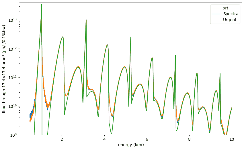
The main modus operandi of xrt synchrotron sources is to provide Monte Carlo rays or wave samples. For comparing our sources with other codes – all of them are fully deterministic, being defined on certain meshes – we also supply mesh methods such as intensities_on_mesh, power_vs_K and tuning_curves. Note that we do not provide any internal mesh optimization, as these mesh functions are not our core objectives. Instead, the user themself should care about the proper mesh limits and step sizes. In particular, the angular meshes must be wider than the electron beam divergences in order to convolve the field distribution with the electron distribution of non-zero emittance. The above mentioned mesh methods will print a warning (new in version 1.3.4) if the requested meshes are too narrow.

If you want to calculate flux through a narrow aperture, you first calculate intensities_on_mesh on wide enough angular meshes and then slice the intensity down to the needed aperture size. An example of such calculations is given in tests/raycing/test_undulator_on_mesh.py which produces the following plot (for a BESSY undulator, zero energy spread, as Urgent cannot take account of it):

Undulator spectrum across a harmonic

The above six classes result in ray distributions with the density of rays proportional to intensity. This requires an algorithm of Monte Carlo ray sampling that needs a 3D (two directions + energy) intensity distribution. The classes using the external mesh-based codes interpolate the source intensity pre-calculated over the user specified mesh. The latter three classes (internal implementation of synchrotron sources) do not require interpolation, which eliminates two problems: artefacts of interpolation and the need for the mesh optimization. However, this requires the calculations of intensity for each ray.

For bending magnet and wiggler sources these calculations are not heavy and are actually faster than 3D interpolation. See the absence of interpolation artefacts in Synchrotron sources in the gallery.

For an undulator the calculations are much more demanding and for a wide angular acceptance the Monte Carlo ray sampling can be extremely inefficient. To improve the efficiency, a reasonably small acceptance should be considered.

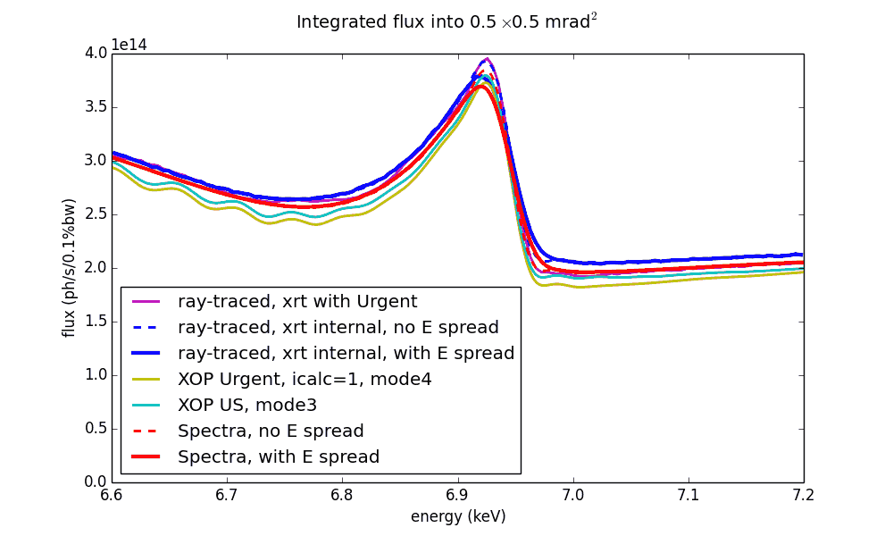
There are several codes that can calculate undulator spectra: [Urgent], [US], [SPECTRA]. There is a common problem about them that the energy spectrum may get strong distortions if calculated with a sparse spatial and energy mesh. SPECTRA code seems to provide the best reference for undulator spectra, which was used to optimize the meshes of the other codes. The final comparison of the resulted undulator spectra around a single harmonic is shown on the left.

[US] (1,2)

R. J. Dejus, US: Program to calculate undulator spectra. Part of XOP.

[SPECTRA] (1,2,3,4,5)

T. Tanaka and H. Kitamura, SPECTRA - a synchrotron radiation calculation code, J. Synchrotron Radiation 8 (2001) 1221-8.

Note

If you are going to use UndulatorUrgent, you should optimize the spatial and energy meshes! The resulted ray distribution is strongly dependent on them, especially on the energy mesh. Try different numbers of points and various energy ranges.

Undulator spectrum at very high energies

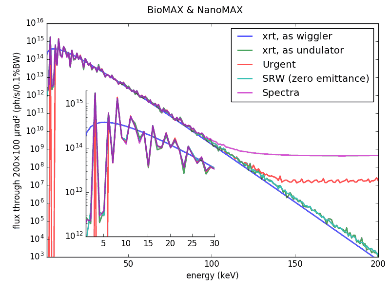
The codes [Urgent] and [SPECTRA] result in saturation at high energies (see the image on the left) thus leading to a divergent total power integral. The false radiation has a circular off-axis shape. To the contrary, xrt and [SRW] flux at high energies vanishes and follows the wiggler approximation. More discussion will follow in a future journal article about xrt.

[SRW] (1,2,3)

O. Chubar, P. Elleaume, Accurate And Efficient Computation Of Synchrotron Radiation In The Near Field Region, proc. of the EPAC98 Conference, 22-26 June 1998, p.1177-1179.

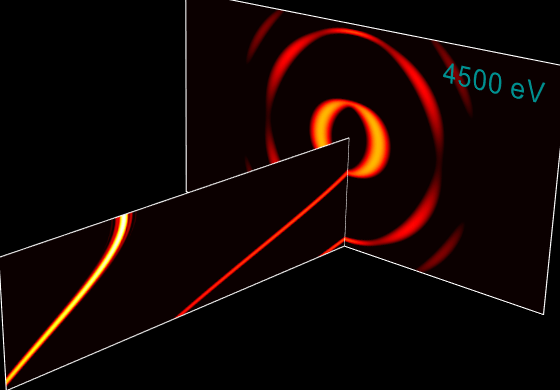
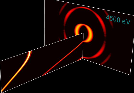
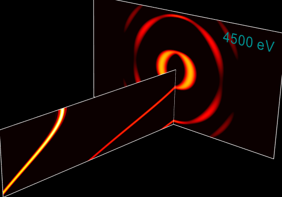
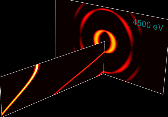
Single-electron and multi-electron undulator radiation

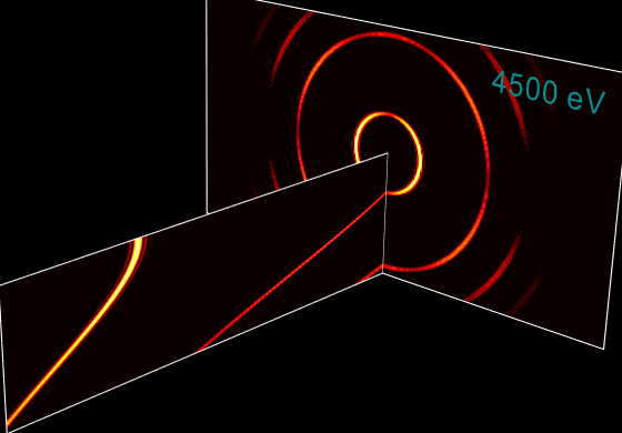
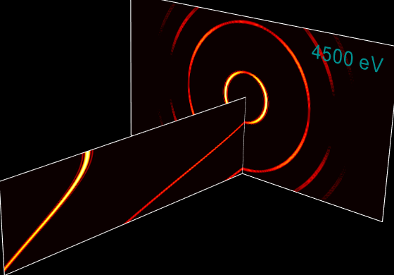
Here we compare single-electron and multi-electron (i.e. with a finite electron beam size and energy spread) undulator radiation, as calculated by xrt and [SRW]. The calculations are done on a 3D mesh of energy (the long axis on the images below) and two transverse angles. Notice also the duration of execution given below each image. The 3D mesh was the following: theta = 321 point, -0.3 to +0.3 mrad, psi = 161 point, -0.15 to +0.15 mrad, energy: 301 point 1.5 to 4.5 keV.

	SRW	xrt
single electron
	execution time 974 s	execution time 17.4 s
non-zero emittance
	execution time 65501 s (sic)	execution time 18.6 s
non-zero emittance, non-zero energy spread
	execution time 66180 s (sic)	execution time 216 s

Undulator spectrum with tapering

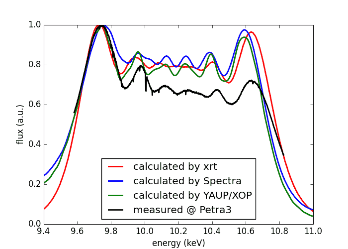
The spectrum can be broadened by tapering of the magnetic gap. The figure on the left shows a comparison of xrt with [SPECTRA], [YAUP] and experimental measurements [exp_taper]. The gap values and the taper were slightly varied in all three codes to reach the best match with the experimental curve. We had to do so because in the other codes taper is not clearly defined (where is the gap invariant – at the center or at one of the ends?) and also because the nominal experimental gap and taper are not fully trustful.

[YAUP]

B. I. Boyanov, G. Bunker, J. M. Lee, and T. I. Morrison, Numerical Modeling of Tapered Undulators, Nucl. Instr. Meth. A339 (1994) 596-603.

[exp_taper]

Measured on 27 Nov 2013 on P06 beamline at Petra 3, R. Chernikov and O. Müller, unpublished.

The source code is in examples/withRaycing/01_SynchrotronSources

Notice that not only the band width is affected by tapering. Also the transverse distribution attains inhomogeneity which varies with energy, see the animation below. Notice also that such a picture is sensitive to emittance; the one below was calculated for the emittance of Petra III ring.

Undulator spectrum in transverse plane

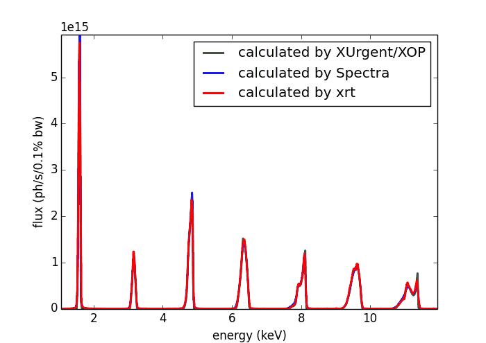
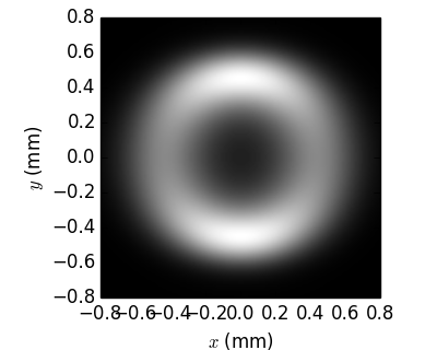
The codes calculating undulator spectra – [Urgent], [US], [SPECTRA] – calculate either the spectrum of flux through a given aperture or the transversal distribution at a fixed energy. It is not possible to simultaneously have two dependencies: on energy and on transversal coordinates.

Whereas xrt gives equal results to other codes in such univariate distributions as flux through an aperture:

… and transversal distribution at a fixed energy:

	SPECTRA	xrt
E = 4850 eV (3rd harmonic)
E = 11350 eV (7th harmonic)

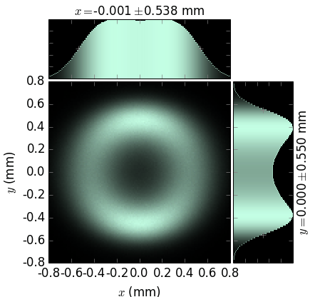
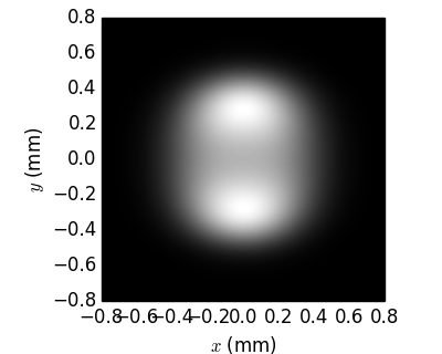
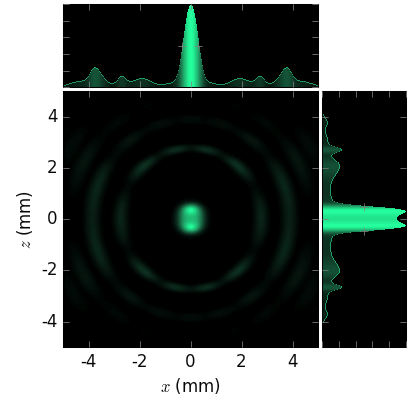
…, xrt can combine the two distributions in one image and thus be more informative:

	zoom in	zoom out
E ≈ 4850 eV (3rd harmonic)
E ≈ 11350 eV (7th harmonic)

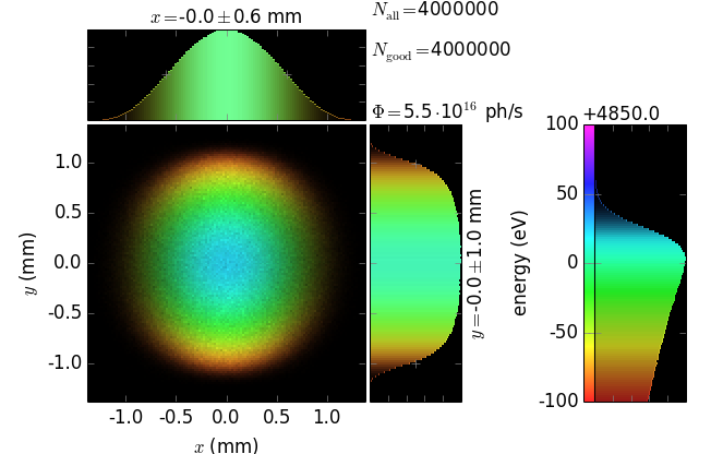
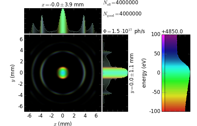
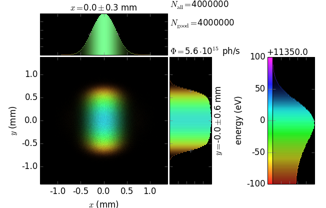
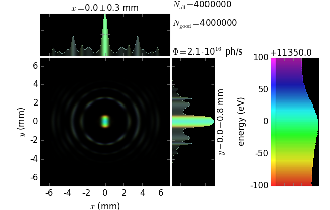
In particular, it is seen that divergence strongly depends on energy, even for such a narrow energy band within one harmonic. It is also seen that the maximum flux corresponds to slightly off-axis radiation (greenish color) but not to the on-axis radiation (bluish color).

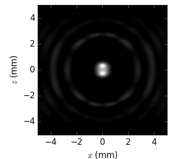
Undulator radiation in near field

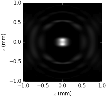
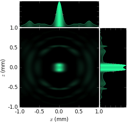
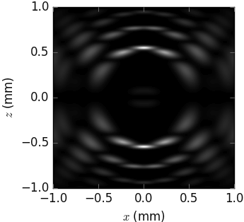
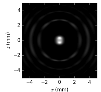
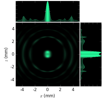
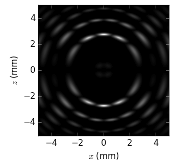
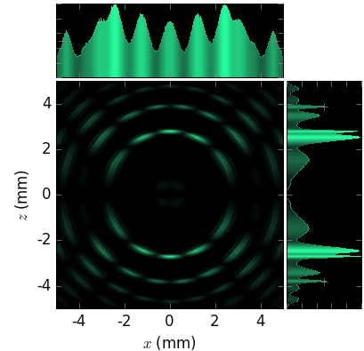
Notice that on the following pictures the p-polarized flux is only ~6% of the total flux.

at 5 m	SPECTRA	xrt
far field at 5 m, full flux
far field at 5 m, p-polarized
near field at 5 m, full flux
near field at 5 m, p-polarized

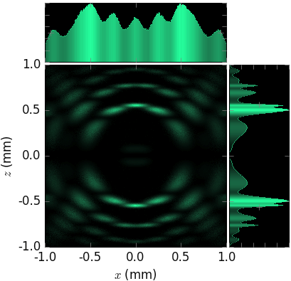
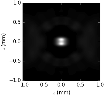
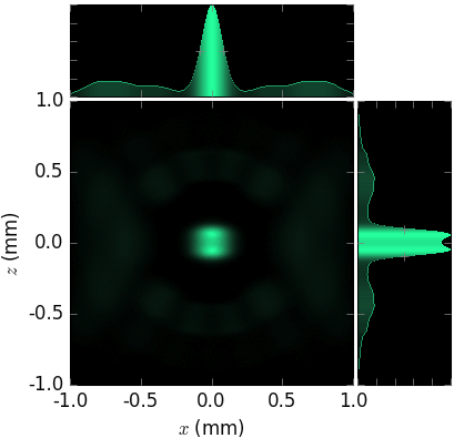
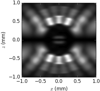
at 25 m	SPECTRA	xrt
far field at 25 m, full flux
far field at 25 m, p-polarized
near field at 25 m full flux
near field at 25 m, p-polarized

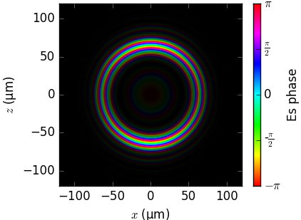
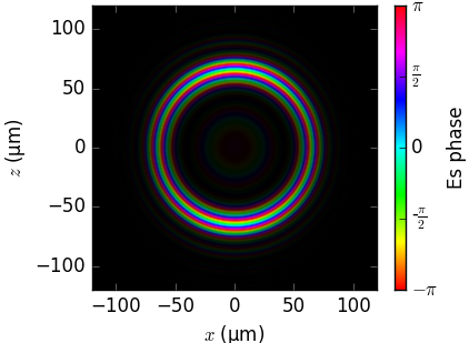
Field phase in near field

The phase of the radiation field on a flat screen as calculated by the three codes is compared below. Notice that the visualization (brightness=intensity, color=phase) is not by SRW and SPECTRA but was done by us.

SRW [SRW]	SPECTRA	xrt

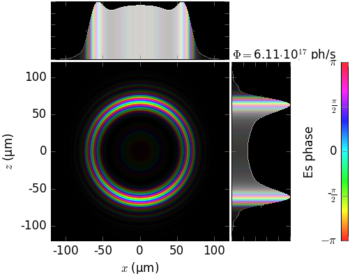
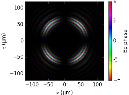
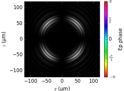
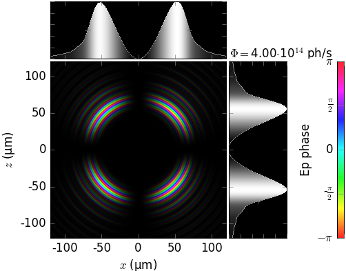
Undulator source size dependent on energy spread and detuning

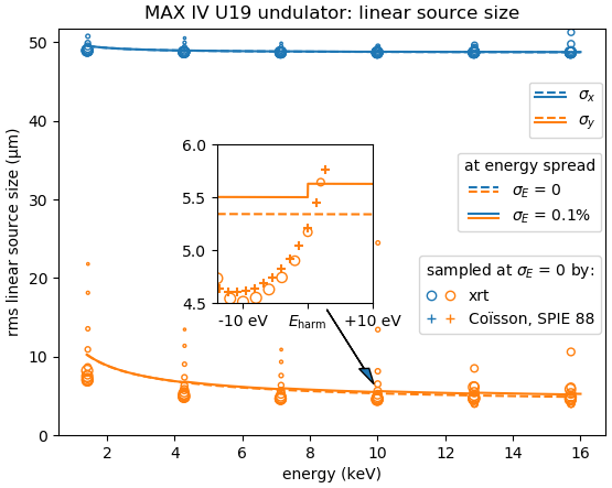
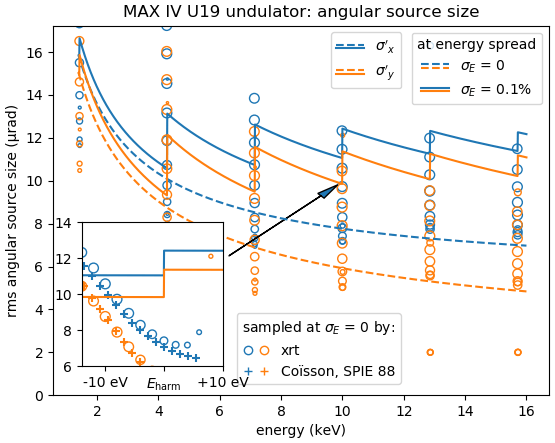
The linear and angular source sizes, as calculated with equations from [TanakaKitamura] (summarized here) for a U19 undulator in MAX IV 3 GeV ring (\(E_1\) = 1429 eV) with \(\varepsilon_x\) = 263 pmrad, \(\varepsilon_y\) = 8 pmrad, \(\beta_x\) = 9 m and \(\beta_y\) = 2 m, are shown below. Energy spread mainly affects the angular sizes and not the linear ones.

The calculated sizes were further compared with those of the sampled field (circles) at variable energies around the nominal harmonic positions, i.e. at so called undulator detuning. To get the photon source size distribution, the angular distributions of Es and Ep field amplitudes were Fourier transformed, as described in [Coïsson]. The sampled field sizes strongly vary due to undulator detuning, as is better seen on the magnified insets. The size variation by detuning is the underlying reason for the size dependence on energy spread: with a non-zero energy spread the undulator becomes effectively detuned for some electrons depending on their velocity.

The size of the circles is proportional to the total flux normalized to the maximum at each respective harmonic. It sharply decreases at the higher energy end of a harmonic and has a long tail at the lower energy end, in accordance with the above examples.

The effect of energy detuning from the nominal undulator harmonic energy on the photon source size is compared to the results by Coïsson [Coïsson] (crosses in the figures below). He calculated the sizes for a single electron field, and thus without emittance and energy spread. For comparison, we also sampled the undulator field at zero energy spread and emittance.

[Coïsson] (1,2)

R. Coïsson, Effective phase space widths of undulator radiation, Opt. Eng. 27 (1988) 250–2.