Introduction: coordinate systems, units and script usage

Coordinate systems

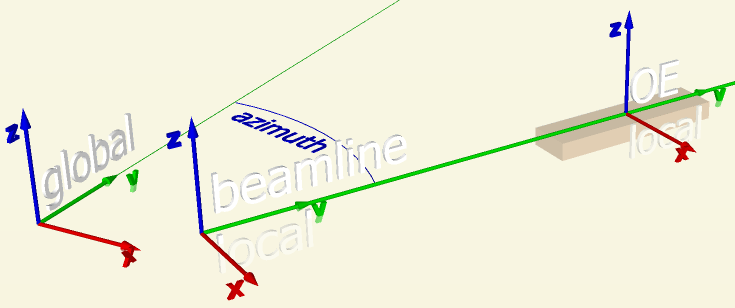
The following coordinate systems are considered (always right-handed):

1. The global coordinate system. It is arbitrary (user-defined) with one requirement driven by code simplification: Z-axis is vertical. For example, the system origin of Alba synchrotron is in the center of the ring at the ground level with Y-axis northward, Z upright and the units in mm.

   Note

   The positions of all optical elements, sources, screens etc. are given in the global coordinate system. This feature simplifies the beamline alignment when 3D CAD models are available.

2. The local systems.

   1. of the beamline. The local Y direction (the direction of the source) is determined by azimuth parameter of BeamLine – the angle measured cw from the global Y axis. The local beamline Z is also vertical and upward. The local beamline X is to the right. At azimuth = 0 the global system and the local beamline system are parallel to each other. In most of the supplied examples the global system and the local beamline system coincide.

   2. of an optical element. The origin is on the optical surface. Z is out-of-surface. At pitch, roll and yaw all zeros the local oe system and the local beamline system are parallel to each other.

      Note

      Pitch, roll and yaw rotations (correspondingly: Rx, Ry and Rz) are defined relative to the local axes of the optical element. The local axes rotate together with the optical element!

      Note

      The rotations are done in the following default sequence: yaw, roll, pitch. It can be changed by the user for any particular optical element. Sometimes it is necessary to define misalignment angles in addition to the positional angles. Because rotations do not commute, an extra set of angles may become unavoidable, which are applied after the positional rotations. See OE.

      The user-supplied functions for the surface height (z) and the normal as functions of (x, y) are defined in the local oe system.

   3. of other beamline elements: sources, apertures, screens. Z is upward and Y is along the beam line. The origin is given by the user. Usually it is on the original beam line.

xrt sequentially transforms beams (instances of Beam) – containers of arrays which hold beam properties for each ray. Geometrical beam properties such as x, y, z (ray origins) and a, b, c (directional cosines) as well as polarization characteristics depend on the above coordinate systems. Therefore, beams are usually represented by two different objects: one in the global and one in a local system.

Units

For the internal calculations, lengths are assumed to be in mm, although for reflection geometries and simple Bragg cases (thick crystals) this convention is not used. Angles are unitless (radians). Energy is in eV.

For plotting, the user may select units and conversion factors. The latter are usually automatically deduced from the units.

Beam categories

Each ray in the beam carries an integer state defined by its propagation status:

0: undefined

No valid propagation state is assigned. This is used for newly created beams.

1: good

Intersected the element within its working optical area.

2: out

Intersected the physical surface outside the working optical area, i.e. outside of a metal stripe on a mirror.

3: over

Propagated past the element without intersection.

-NN: dead

Lost (absorbed) at the beamline element with lostNum=-NN. Dead rays remain in the beam arrays but are excluded from further propagation.

This distinction simplifies the adjustment of entrance and exit slits. The user supplies physical and optical limits, where the latter is used to define the out category (for rays between physical and optical limits). An alarm is triggered if the fraction of dead rays exceeds a specified level.

Scripting in python

The user of raycing must do the following:

1. Instantiate class BeamLine and fill it with sources, optical elements, screens etc.

2. Create a module-level function that returns a dictionary of beams – the instances of Beam. Assign this function to the module variable xrt.backends.raycing.run.run_process. The beams should be obtained by the methods shine() of a source, expose() of a screen, reflect() or multiple_reflect() of an optical element, propagate() of an aperture.

3. Use the keys in this dictionary for creating the plots (instances of XYCPlot). Note that at the time of instantiation the plots are just empty placeholders for the future 2D and 1D histograms.

4. Run run_ray_tracing() function for the created plots.

Additionally, the user may define a generator that will run a loop of ray tracing jobs for changing geometry settings (mimics a real scan) or for different material properties etc. The generator should modify the beamline elements and output file names of the plots before yield. After the yield the plots are ready and the generator may use their fields, e.g. intensity or dE or dy or others to prepare a scan plot. Typically, this sequence is contained within a loop; after the loop the user may prepare the final scan plot using matplotlib functionality. The generator is passed to run_ray_tracing() as a parameter.

Consider an example of a generator:

def energy_scan(beamLine, plots, energies):
    flux = np.zeros_like(energies)
    try:
        trapz = np.trapezoid
    except AttributeError:
        trapz = np.trapz
    for ie, e in enumerate(energies):
        print(f'energy {e:.1f} eV, {ie+1} of {len(energies)}')
        beamLine.fixedEnergy = e
        beamLine.source.eMin = e - 0.5  # defines 1 eV energy band
        beamLine.source.eMax = e + 0.5
        for plot in plots:
            plot.saveName = [plot.baseName + f'-{ie}-{e:.1f}eV.png']

        yield
        # now all plots for this scan point are ready
        flux[ie] = plot.flux

    # now the whole scan is complete
    integratedFlux = trapz(flux, energies)
    print(f'total flux = {integratedFlux:.3g} ph/s')

    with open("ray_tracing_c.pickle", 'wb') as f:
        pickle.dump([energies, flux, integratedFlux], f)

    plt.plot(energies, flux)
    plt.show()

… and an example of passing this generator to run_ray_tracing():

def ray_study(nrays, repeats):
    beamLine = build_beamline(nrays)
    plots = define_plots(beamLine)
    energies = np.linspace(11800, 12600, 401)
    xrtr.run_ray_tracing(
        plots, repeats=repeats, beamLine=beamLine,
        generator=energy_scan, generatorArgs=[beamLine, plots, energies])

Find more generators in the supplied examples.

class xrt.backends.raycing.BeamLine(azimuth=0.0, height=0.0, alignE='auto', fileName=None, name='beamLine', description='', **kwargs)

Container class for beamline components. It also defines the beam line direction and height.

__init__(azimuth=0.0, height=0.0, alignE='auto', fileName=None, name='beamLine', description='', **kwargs)

azimuth: float

Is counted in cw direction from the global Y axis. At azimuth = 0 the local Y coincides with the global Y.

height: float

Beamline height in the global system.

alignE: float or ‘auto’

Energy for automatic alignment in [eV]. If ‘auto’, alignment energy is defined as the middle of the Source energy range. Plays a role if the pitch or bragg parameters of the energy dispersive optical elements were set to ‘auto’.